SUPPLEMENTARY INFORMATION
doi:10.1038/nature09696
INTRODUCTION
This discussion is organised into three parts. The first presents the mathematical description of the hyperpolarisation sequence applied to the thermal density matrix. The second
section introduces the PPT criterion and applies it to derive entanglement thresholds for a
selection of preparation strategies. The third section describes the analysis used to collect
the final density matrix, error ranges, and a discussion on fidelities.
HYPERPOLARISATION
Si:P is described by an isotropic spin Hamiltonian (in angular frequency units):
 · I,

H0 = ωe Sz − ωI Iz + a· S
(1)
where ωe = gβB0 / and ωI = gI βn B0 / are the electron and nuclear Zeeman frequencies, g
and gI are the electron and nuclear g-factors, β and βn are the Bohr and nuclear magnetons,
 is Planck’s constant and B0 is the magnetic field applied along z-axis in the laboratory
frame. Sx,y,z = σx,y,z ⊗ I2 and Ix,y,z = I2 ⊗ σx,y,z .
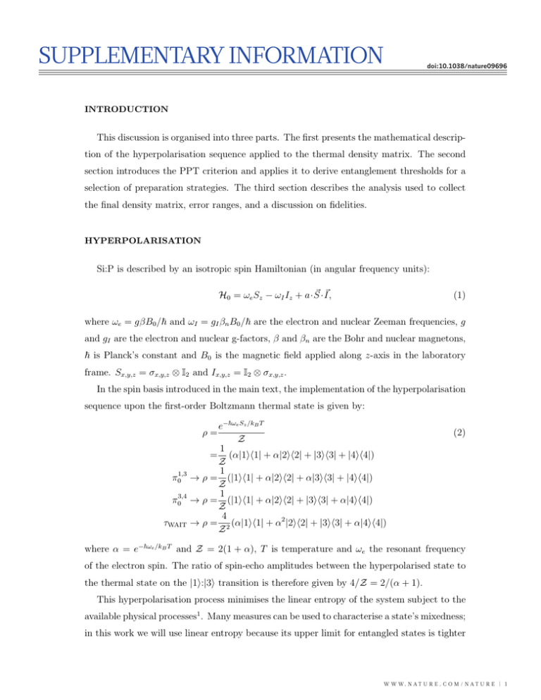
In the spin basis introduced in the main text, the implementation of the hyperpolarisation
sequence upon the first-order Boltzmann thermal state is given by:
e−ωe Sz /kB T
Z
1
= (α|11| + α|22| + |33| + |44|)
Z
1
→ ρ = (|11| + α|22| + α|33| + |44|)
Z
1
→ ρ = (|11| + α|22| + |33| + α|44|)
Z
4
→ ρ = 2 (α|11| + α2 |22| + |33| + α|44|)
Z
ρ=
π01,3
π03,4
τWAIT
(2)
where α = e−ωe /kB T and Z = 2(1 + α), T is temperature and ωe the resonant frequency
of the electron spin. The ratio of spin-echo amplitudes between the hyperpolarised state to
the thermal state on the |1:|3 transition is therefore given by 4/Z = 2/(α + 1).
This hyperpolarisation process minimises the linear entropy of the system subject to the
available physical processes1 . Many measures can be used to characterise a state’s mixedness;
in this work we will use linear entropy because its upper limit for entangled states is tighter
2
w w w . n a t u r e . c o m / NATURE | 1
RESEARCH SUPPLEMENTARY INFORMATION
than the von Neumann entropy limit2 . The linear entropy is given by
SL (ρ) ≡
N
[1 − Tr(ρ2 )]
N −1
(3)
where N is the dimension of the Hilbert space. The linear entropies of the thermal and
hyperpolarised states are given by
2(1 + 4α + α2 )
3(1 + α)2
16α(1 + α + α2 )
SL (ρhyperpol ) =
3(1 + α)4
SL (ρthermal ) =
The linear entropy decrease is:
SL (ρthermal ) − SL (ρhyperpol ) =
2(1 − α)2 (1 + α2 )
3(1 + α)4
(4)
ENTANGLEMENT THRESHOLDS
The PPT criterion states that, for a bipartite spin 1/2 system, a state is entangled if
and only if its partial transpose has a negative eigenvalue. Explicitly, let us consider a state
within the bipartite Hilbert space H = HA ⊗ HB expressed in the form
ρ=

i,j,k,l
pij,kl |ij| ⊗ |kl|
where the first pair of indices range over HA and the second pair over HB . The partial
transpose of this state is given by
ρTB =

i,j,k,l
pij,kl |ij| ⊗ (|kl|)T =

i,j,k,l
pij,kl |ij| ⊗ |lk|.
This operation is a transposition of HB but not HA . If a state in H is a product state,
applying such an operation would produce a physically allowed density matrix. Applying
the PPT to an entangled state would instead result in an unphysical state, which manifests
as a negative eigenvalue. Because ρTA = (ρTB )T , the PPT result does not depend upon
which subspace is transposed.
As discussed in the text, our target entangled state was optimally chosen within the limits
of the state’s linear entropy. We can apply the entangling sequence to the hyperpolarised
3
2 | WWW. NATURE . COM / NATURE
SUPPLEMENTARY INFORMATION RESEARCH
state expressed in the form of a density matrix in the {|1 , |2 , |3 , |4} basis.

α 0 0 0

 0 α2


0 0

0 0

1+α

2 
 0
→ρ= 2
Z  0

1−α
4
ρ= 2
Z
 π 1,3
2
π/2
, π03,4


0 0


1 0

0 α
0
0 1−α


0 


2α 0 

0 1+α
2α2 0
0
0
(5)
The partial transpose of this state is:

1+α
2
Z2

 0


 0

0
0
0
2α2 1 − α
1−α
2α
0
0
0


0 


0 

1+α
and the eigenvalues of this matrix has a zero crossing when
α3 − (1 − α)2 /4 = 0
or when α ≈ 0.432.
It is worth briefly considering the crossing-points for other preparation strategies, in each
case using the optimal entangling sequence described above. Three examples include i) the
pseudopure preparation scheme applied to the thermal state ii) the thermal state with no
preparation and iii) the pseudopure preparation scheme applied to the hyperpolarised state.
For i), the prepared pseudopure state has the form

(1 + 2α)/3
ρpp
1
=
Z






0
0
0
0
(1 + 2α)/3 0
0
0
0
1
0
0
0
0 (1 + 2α)/3







This initial state produces the maximal amount of entanglement when arranged in the form
4
w w w . n a t u r e . c o m / NATURE | 3
RESEARCH SUPPLEMENTARY INFORMATION
equivalent under local unitaries to


(4 + 2α)/6
0
0
(2 − 2α)/6



0
(1
+
2α)/3
0
0
1 


ρpp = 


Z
0
0
(1
+
2α)/3
0


(2 − 2α)/6
0
0
(4 + 2α)/6
The partial transpose of this matrix has a zero crossing when
2α + α2 = 0
and so the only ‘physical’ zero crossing occurs at α = 0. Of course, these calculations assume
that the nuclear spin polarisation is negligible; in the regime of α ≈ 0 the polarisation of
the nucleus would have to be considered in this calculation. This would allow for a small
but nonzero threshold for α, dependent upon the nuclear spin isotope.
For ii), the maximally entangled state is equivalent under local unitaries to


(1 + α)/2 0 0 (1 − α)/2



0
α 0
0
1 


ρpp = 



Z
0
0 1
0


(1 − α)/2 0 0 (1 + α)/2
√
The partial transpose of this matrix has a positive zero crossing when α = −3 + 2 2, so
entanglement is possible below α ≈ 0.17.
For iii), the maximally entangled state is equivalent under local unitaries to


(3 + 2α + α2 )/6
0
0
(3 − 2α − α2 )/6



0
α(2 + α)/3
0
0
4 


ρpp = 2 


Z 
0
0
α(2
+
α)/3
0


2
2
0
0
(3 + 2α + α )/6
(3 − 2α − α )/6
√
The partial transpose of this matrix has a positive zero crossing when α = 2 − 1, and so
entanglement is possible below α ≈ 0.4142.
DENSITY MATRIX CALCULATIONS
We used phase (Z) rotations to probe the existence of coherences without disturbing the
state populations, which were measured separately by mapping pairs of population differences into the Sx observable. In typical electron spin resonance experiments, phase rotations
5
4 | WWW . NATURE . COM / NATURE
SUPPLEMENTARY INFORMATION RESEARCH
FIG. 1: Geometric Phase Rotations Geometric Z-gates can be applied to a single spin using
two consecutive π pulses along different axes. The black arrows at each step illustrate the applied
rotation to the Bloch sphere, and the colouring displays this rotation. Three sample geometric
Z-gate rotations are shown along the bottom.
are not directly available operations; they can be implemented with various strategies including the use of off-resonant pulses and appropriate delays, phase-shifted final reference
frames3 and composite rotations made up of pure X and Y rotations of variable length4 . In
this work, we follow an approach inspired by the Aharonov-Anandan geometric phase gate5
and apply two selective MW or RF π pulses of differing phases. Given the larger Hilbert
space of this two-spin system, and the fact that we are applying selective rotations that
cannot be understood in terms of the independent manipulation of either spin, the most
instructive way to appreciate the effect of this gate is to examine the phase acquired by each
eigenstate under the rotation (see Figure 2 of the main text). However, for a single spin 1/2,
the same gate has a convenient visual representation that is illustrated in Figure 1 in terms
of the rotation of the Bloch sphere.
To calculate the final density matrix we first constructed the pseudo-pure density matrix. A baseline measurement was taken as an average of 2000 samples, and all datasets
were baseline-corrected before processing. The population differences were measured by an
average of 100 samples and scaled with respect to a measured thermal amplitude (also taken
6
w w w . n a t u r e . c o m / NATURE | 5
RESEARCH SUPPLEMENTARY INFORMATION
as an average over 100 samples), and adjusted to have unit trace with the addition of an
appropriately scaled identity matrix.
The coherence-measurement pulse sequences were all individually tested by verifying their
output frequencies when applied to their target coherences. Upper diagonal elements were
gathered and their conjugate values populated the lower diagonal elements. The coherences
were collected with 128 points and baseline-corrected before being Fourier transformed and
normalised with respect to the thermal amplitude. A narrow integral over the appropriate
frequency position was made to measure the coherences. The frequencies were chosen such
that all frequency peaks were well-resolved with a 128-point Fourier transform.
The calculated pseudopure matrix ρpp was added to the appropriate amount of identity
matrix I as determined by a spin-temperature measurement, where e−ωs /kb T = α ≤ 0.217.
The explicit reconstruction is given by
ρF = [α/(2(1 + α))]I + [(1 − α)/((1 + α))]ρpp
� �√
√ 2
ρ2 ρ1 ρ2
There are two conventional measures6,7 of state fidelity, F(ρ1 , ρ2 ) = Tr

or alternatively the more generous measure F(ρ1 , ρ2 ). When applied to physically allowed
states, both measures are non-negative and reach a maximum value of 1 when ρ1 = ρ2 . The
fidelity used in the main text calculates F when comparing the gathered density matrix
with the target density matrix (calculated by Equation 5 with α = 0.217). This measure
√
yields a fidelity of 0.982(2), while the often-used alternative measure F displays a fidelity
of 0.991(2) with the target state. We can also compare the gathered density matrix to the
√1 (|0000|
2
+ |1111|) given by Equation 5 with α = 0. The adopted
√
fidelity F reveals a fidelity of 0.68(2), while the more generous F produces a fidelity of
ideal Bell state ρB =
0.82(1) with the pure Bell state.
The errors corresponding to each density matrix element were calculated according to
the standard error of the measurement taken. For the populations this consisted of the
standard error of the direct difference measurements; for the coherences this consisted of the
standard error of the Fourier-transformed signal over the integral peak width. These density
matrix element errors were transformed into final negativity, concurrence and fidelity errors
by Monte Carlo generation of density matrices. The generated matrices deviated from the
measured matrix in each element by an amount chosen randomly from a normal distribution
whose standard deviation matched that elements’ error. Once re-normalised, unphysical
7
6 | WWW . NATURE . COM / NATURE
SUPPLEMENTARY INFORMATION RESEARCH
matrices were discarded and statistics on physical matrices were collected. In total, 212
matrices were used to compile the final errors.
[1] Schulman, L. J., Mor, T. & Weinstein, Y. Physical Limits of Heat-Bath Algorithmic Cooling.
Phys. Rev. Lett. 94 (2005).
[2] Wei, T.-C. Maximal entanglement versus entropy for mixed quantum states. Phys. Rev. A 67
(2003).
[3] Mehring, M., Mende, J. & Scherer, W. Entanglement between an Electron and a Nuclear Spin
1/2. Phys. Rev. Lett. 90, 153001 (2003).
[4] Suter, D., Mueller, K. T. & Pines, A. Study of the Aharonov-Anandan quantum phase by
NMR interferometry. Phys. Rev. Lett. 60, 1218–1220 (1988).
[5] Aharonov, Y. & Anandan, J. Phase change during a cyclic quantum evolution. Phys. Rev.
Lett. 58, 1593–1596 (1987).
[6] Jozsa, R. Fidelity for mixed quantum states. Journal of Modern Optics (1994).
[7] DiCarlo, L. et al. Demonstration of two-qubit algorithms with a superconducting quantum
processor. Nature 460, 240–244 (2009).
w w w . n a t u r e . c o m / NATURE | 7