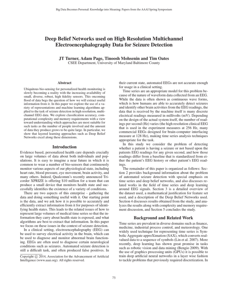
Big Data Becomes Personal: Knowledge into Meaning: Papers from the AAAI Spring Symposium
Deep Belief Networks used on High Resolution Multichannel
Electroencephalography Data for Seizure Detection
JT Turner, Adam Page, Tinoosh Mohsenin and Tim Oates
CSEE Department, University of Maryland Baltimore County
Abstract
their current state, automated EEGs are not accurate enough
for usage in a clinical setting.
Time series are an appropriate model for this problem because of the nature of waveform data collected from an EEG.
While the data is often shown as continuous wave forms,
which is how humans are able to accurately detect seizures
and identify other brain activities from the EEG readings, the
data that is received by the machine itself is many discrete
electrical readings measured in millivolts (mV). Depending
on the design of the actual system itself, the number of readings per second (Hz) varies (the high resolution clinical EEG
that is used in the experiment measures at 256 Hz, many
commercial EEGs designed for brain-computer interfacing
measure at 128 Hz), making time series analysis techniques
appropriate for the task.
In this study we consider the problem of detecting
whether a patient is having a seizure or not based upon the
patients EEG readings for any given second, and how those
readings differ from a baseline that is standardized from either the patient’s EEG history or other patient’s EEG readings.
The remainder of this paper is organized as follows: Section 2 provides background information about the problem
of automated seizure detection with special emphasis on
time series and deep belief networks, and also discusses related works in the field of time series and deep learning
around EEG signals. Section 3 is a detailed overview of
the dataset used, a mathematical justification for feature set
used, and a description of the Deep Belief Networks used.
Section 4 discusses results obtained from the study, and analyzes the results along with complexity and memory requirement discussion, and Section 5 concludes the study.
Ubiquitous bio-sensing for personalized health monitoring is
slowly becoming a reality with the increasing availability of
small, diverse, robust, high fidelity sensors. This oncoming
flood of data begs the question of how we will extract useful
information from it. In this paper we explore the use of a variety of representations and machine learning algorithms applied to the task of seizure detection in high resolution, multichannel EEG data. We explore classification accuracy, computational complexity and memory requirements with a view
toward understanding which approaches are most suitable for
such tasks as the number of people involved and the amount
of data they produce grows to be quite large. In particular, we
show that layered learning approaches such as Deep Belief
Networks excel along these dimensions.
Introduction
Evidence based, personalized health care depends crucially
on large volumes of data about both individuals and populations. It is easy to imagine a near future in which it is
common to wear a number of bio-sensors that continuously
monitor various aspects of our physiological state, including
heart rate, blood pressure, eye movement, brain activity, and
many others. Indeed, Qualcomm’s recently announced Tricorder XPRIZE is offering $10 million for a team that can
produce a small device that monitors health state and successfully identifies the existence of a variety of conditions.
There are two aspects of this enterprise - gathering the
data and doing something useful with it. Our starting point
is the data, and we ask how it is possible to accurately and
efficiently extract information from it for purposes of identifying health states. This leads to the related issues of how to
represent large volumes of medical time series so that the information they carry about health state is exposed, and what
algorithms are best to extract that information. In this paper
we focus on these issues in the context of seizure detection.
In a clinical setting, electroencephalography (EEG) can
be used to survey electrical activity in the brain, which can
be used to diagnose and monitor abnormal brain functioning. EEGs are often used to diagnose certain neurological
conditions such as seizures. Automated seizure detection is
still a difficult task, and often produced false positives. In
Background and Related Work
Time series are prevalent in diverse domains such as finance,
medicine, industrial process control, and meteorology. One
widely used technique for representing time series is Symbolic Aggregate approXimation (SAX), which converts realvalued data to a sequence of symbols (Lin et al. 2007). More
recently, deep learning has shown great promise in tasks
such as robotic vision and data mining (Bengio 2009). With
the use of graphics processing units (GPUs) it is possible to
train deep artificial neural networks in a layer wise fashion
to tackle problems that previously required discretization. In
c 2014, Association for the Advancement of Artificial
Copyright Intelligence (www.aaai.org). All rights reserved.
75
the remainder of this section we introduce terminology, review the deep learning methods used in this work, and discuss related work in the domain of seizure detection using
machine learning.
one group of nodes being the visible layer of the RBM,and
the other group of nodes being the hidden layer of the RBM.
h_0
h_1
Hidden Layer
Multichannel Time Series
Let T be a time series representing an EEG that samples at
a rate of H Hz over C channels for S seconds. The multichannel time series can be denoted as follows (where Xc,s,h
is the reading of the cth channel on the hth sample of the sth
second, measured in mV):
T = (x0,0,0 ,
x0,0,1 , ..., x0,0,H−1 ),
(x1,0,0 ,
...
Visible Layer
v_0
xC−1,0,1 , ..., xC−1,0,H−1 ) ,
...
(x0,S−1,0 ,
x0,S−1,1 , ..., x0,S−1,H−1 ),
(x1,S−1,0 ,
...
x1,S−1,1 , ..., x1,S−1,H−1 ),
(xC−1,S−1,0 ,
xC−1,S−1,1 , ..., xC−1,S−1,H−1 )
v_2
Figure 2: The hidden node pointed to by the arrow is a column of the 3×2 weight matrix W , and a scalar of the weight
vector h.
The concept of a node in an RBM is an abstraction to help
us visualize them. A ”hidden node” is just the column Wj of
W , and the scalar hj of h; similarly, a ”visible node” is the
row Wi of W , and the scalar vi of v.
What the RBM does is to learn the probability distribution
of the inputs. It does this in a stochastic manner such that
the machine is less likely to be entrapped on local maxima.
Two other important components of RBMs are that they are
able to facilitate dimensionality reduction or expansion as is
needed for the proper level of abstraction, and that they can
be trained in a greedy manner one layer at a time.
The ability to change the dimensionality of the input is a
powerful idea, and the basis for the success deep learning
methods have in such areas as robotic vision. DBNs morph
the input space into a larger space where abstract objects
such as lines, edges, and corners can be formed, and then
furthermore constricting that space tighter so that high level
objects such as smooth valleys, peaks, and flat lines can be
observed by the machine. The artificial neural network generated by the stacking of RBMs is capable of taking raw data
(pixels, or in our case electrical signals), and transforming it
into data that is useful for the machine to use and process.
Training deep belief networks is best done one layer at a
time, in a layerwise manner (Bengio et al. 2007). RBM r0
can be completely trained to gather the structure of the underlying data independently of r1 , r2 ... , by taking the difference of the positive gradient (which is obtained by computing the outer product of the visible input sample v, and
the sampled hidden layer h), and the negative gradient (obtained by computing the outer product of a reconstruction v 0
(by sampling from h), and h0 (by sampling from v 0 ), and adjusting the matrix W as needed from the difference of these
gradients.
Once every layer of the deep belief network has been
trained using the method described above, the output layer
of the final RBM can be used as the input to a classifier. For
this study, a simple logistic regression classifier was used,
although an SVM or kNN could easily be used in its place.
x1,0,1 , ..., x1,0,H−1 ),
(xC−1,0,0 ,
v_1
.
This results in a massive amount of high resolution clinical
quality EEG data that is so large that it is both unwieldy and
may dilute information critical to the task of seizure detection. Featurization of the raw data is critical and is discussed
in Section 3.
Classifiers used in this work
Three classifiers are used in this work to compare the detection accuracy and computational and memory requirements.
These classifiers are: K-nearest neighbor (KNN) with 3, 5,
and 7 neighbors, Support Vector Machines (SVM) with sigmoid, radial basis function, and polynomial kernels, and logistic regression. Figure 1 shows a schematic description of
these three classifiers.
Deep Belief Networks
Deep Belief Networks are a new algorithm in the deep learning family, consisting of a set of N Restricted Boltzmann
Machines (RBMs) R = r0 , r1 , ..., rN −1 that are paired with
a classifier C that takes as input the output of the final RBM
and outputs class probabilities. The RBMs are stacked in
such a way that the output layer of the RBM at layer ` − 1
is the input to the RBM at layer `. A deep belief network is
a system of 2 or more RBMs stacked in this way.
The purpose of the RBM is to learn a probability distribution over a set of inputs, and each RBM consists of the following components: a weight matrix W of size i × j, where
i is the number of visible nodes and j is the number of hidden nodes, a visible bias v of length i, and a hidden bias h
of length j. Each RBM is in essence a bipartite graph, with
Related Work
This study builds upon previous studies in the area of seizure
detection, deep belief networks, and time series analysis of
high resolution medical data.
In a study by Wulsin (Wulsin et al. 2011), deep belief networks were also used for analysis of data obtained from an
76
KNN
SVM
Log Reg
Figure 1: The k-Nearest Neighbor (KNN) classifier labels an instance by a majority vote of its k closest neighbors in the instance
space according to some distance function. Support vector machines (SVM) learn linear separators in high-dimensional spaces
that depend on the kernel used such that the separators are often non-linear in the original feature space. Logistic regression
(LR)learns a weight vector that maps instances to class probabilities through a logistic function which, when thresholded,
results in a linear separator.
Features used
EEG. The feature set that we chose to use was borrowed
from a larger set of features used in this study, however this
study attempted to classify anomalous EEG features such as
GPED, PLED, or eye blinks as opposed to seizure detection.
A particularly useful study by Shoeb and Guttag used the
same dataset of seizure patients that were being monitored
by high resolution EEGs after being withdrawn from antiseizure medications (Shoeb 2009). Although using the same
dataset, the Shoeb study extracted a different feature set, and
used a support vector machine as the binary classifier, as opposed to a deep belief network. Furthermore, in this study
the seizure progression was not interrupted, and statistics
were kept on not only the accuracy of seizures detected, but
the amount of time that was taken to detect the seizures by
the support vector machine.
A final study by Oates et al. (Oates et al. 2012) motivated
this study and paper. The paper did not study seizure detection, rather traumatic brain injury outcomes. The Oates
study investigated time series of high resolution medical
data as well, however the data in this study was pulse rate,
and SpO2 levels. The study used a Bag of Patterns approach
to pre-process data to be used in 1NN clustering to clasify
early outcome predictions of patients with traumatic brain
injuries.
In the following definitions, a peak is defined as a reading
that marks the change from a positive to negative derivative,
and a valley is defined as a reading that marks a change
from a negative derivative to a positive derivative. ki will
mark the index of the k th peak of the time series, with a
value of xk(i) . Similarly, vi will mark the ith valley index,
and xv(i) will mark the value of it. Window size is given
by W . Given a single channel time series T , with reading
xi ∀i ∈ T .:
• Area: Area under the wave for the given time series. Computed as:
W −1
1 X
A=
xi .
W i=0
• Normalized Decay: Chance corrected fraction of data that
has a positive or negative derivative. I(x) is a boolean
indicator function, whose value is 1 when true, 0 when
false.
W
−2
X
1
D=|
I(xi+1 − xi < 0) − .5|.
W − 1 i=0
• Line Length: Summation of distance between all consecutive readings.
Method and Approach
`=
W
X
−1|xi − xi−1 |.
i=1
Because using the raw signal input as the input to the deep
belief network or classifiers does not allow for the algorithm
to properly abstract from the raw data, certain features of the
dataset are derived from the raw time series signal. Because
a trained human can look at the EEG wave pattern and determine whether or not a seizure is occurring with close to
perfect accuracy, many of the features extracted are visible
features of the time series such as area under curve, or variation of peaks. The following features were used for detection
of anomalous EEG features in the Wulsin study (Wulsin et
al. 2011).
• Mean Energy: Mean energy of time interval.
E=
W −1
1 X 2
|x |.
W i=0 i
• Average Peak Amplitude: Log base 10 of mean squared
amplitude of the K peaks.
1 K−1
X
PA = log10
x2k(i) .
K i=0
77
• Average Valley Amplitude: Log base 10 of mean squared
amplitude of the V valleys.
VA = log10
−1
1 VX
V
80
60
40
20
0
-20
-40
-60
-80
x2v(i) .
i=0
⟨ D0 , D1 , … , DW ⟩
• Normalized Peak Number: Given K peaks, normalized
peak number is the number of peaks normalized by the
average difference between data readings.
NP = K
1
W −1
W
−2
X
|xi+1 − xi |
−1
Single Channel Raw EEG Data
Simple
Feature Extraction
.
⟨ F 0 , F1 , … , F M⟩
i=0
• Peak Variation: Variation between peaks and valleys
across time (measured in Hz), and electrical signal (measured in mV). In the case where the number of peaks is
not equal to the number of valleys (if an time interval begins or ends during an increase or decrease in data, it is
not recorded as a peak or valley), than the feature with
the least features is used in comparisons between peaks
and valleys. The mean (µ(P V )) and standard deviation
(σ(P V )) of the indicies are given by:
DBN
Feature Classication
Figure 3: Flow diagram of our experiments for seizure detection using two parts.
K−1
1 X
Ki − Vi .
K i=0
v
u
u 1 K−1
X
σ(P V ) = t
(Ki − Vi − µ(P V ))2 .
K − 1 i=0
µ(P V ) =
two different approaches to investigate the seizure detection
accuracy; Part 1 which uses simple features extraction followed by three different classifiers: SVM, KNN and logistic
regression. Part 2 uses simple features extraction followed
by DBN and a classifier which is logistic regression. Figure 3 shows the flow diagram for our experiment approach,
where Di represents the digitized raw EEG data within a 256
window size (W =256) and Fi represents the corresponding
feature for a single channel (N = 9 features).
The difference in readings is given by
K−1
1 X
xk(i) − xv(i) .
K i=0
v
u
u 1 K−1
X
σ(xP V ) = t
(xk(i) − xv(i) − µ(xP V ))2 .
K − 1 i=0
µ(xP V ) =
Design & Parameters for DBN
The deep belief network training program was obtained from
the Theano library from the LISA lab of University of Montreal (Bergstra et al. 2010), with modifications made to save
best models (not only most recent), and improved methods
to allow training progress to be monitored. Training was
done for a significant amount of time to enhance results,
which was possible using GPU calculations which proved
to be much faster than using the CPU alone. The calculations were done on a Dell Precision M4700 model with an
Intel Core i7-3940XM CPU @ 3.00GHz, 16 GB of memory
@ 1866 MHz, and the graphics card used for GPU calculations was an NVIDIA Quadro K2000M with 384 unified
pipelines @ 745 MHz, with 2 GB of video memory.
The input data was changed to the features shown in Secion 3. The EEG that collected the readings sampled from
23 channels at 256 hertz, so using the raw data as input to
the algorithm would prove difficult, as each second would
contain 5,888 distinct EEG readings for the machine to process.
The number of input nodes to the deep belief network were
set at 207, with 2 output nodes to classify a second of EEG
data as a seizure or non seizure. The number of layers, and
number of nodes inside each of the hidden layers of the
The peak variation is calculated as
1
PV =
.
σ(P V )σ(xP V )
• Root Mean Square: The square root of the mean of the
data points squared.
v
u W −1
u 1 X
x2 .
RM S = t
W i=0 i
These nine features were used as the feature space for a
single channel of EEG input. In this study, the high resolution EEG data received from 23 channels, so after featurization, the size of the input vector was 23 ∗ 9 = 207 real
numbered values. Before the raw data was converted to features, the data was normalized, with µ = 0, σ = 1, and
the top 2.5% and bottom 2.5% of values were truncated to
2 and -2 respectively. The normalization was done with respect to each channel individually. Features were then calculated, and then were standardized from [0, 1] for the final input to the deep belief network or a classifier. We used
78
RBMs was determined through extensive trial and error. The
best parameter set was found to be two hidden layers of 500
nodes each. Using CD-1 was found to be sufficient to the
task of building structure for classification, and 25 epochs
were performed on each layer of the RBM in pretraining,
with a learning rate α = .001. After the pretraining process
of abstraction was completed (without the usage of class labels), the logistic regression layer was trained in the finetuning process. 16 iterations of finetuning were completed, with
a learning rate α = .1.
Code for classifying instances given a training model was
trivial, and emphasizes one of the highlights of deep belief
networks. The input to the level k of the network was multiplied by the weight matrix Wk , and added to bias matrix
Wb . The hidden bias and inverted weight matrices used in
the pretraining algorithm are not used, because for classification we do not wish to introduce noise into our sample by
repropogating the input. When the final layer of the DBN is
reached, the argmax of the output layer is taken to assign the
class label.
Figure 4: Comparison of different classifiers when single patient data is used for training and test
Results and Analysis
We used two different approaches to investigate the seizure
detection accuracy: part 1 which uses simple features extraction followed by three different classifiers: SVM, KNN and
logistic regression. Part 2 uses simple features extraction followed by DBN and a classifier, which is logistic regression
in this case.
In addition, two different methods of classification tasks
were done on the data. In one study the same patient was
used for both training, validation, and testing sets. This led
to a much smaller corpus, but had very good results. The
second study involved using all of the other nine patients
with data for training and validation sets, and then using one
patient at a time for a testing set. This allowed for a much
larger corpus for training and testing, but did not produce results as high as the first study. In every study, the majority of
the time, the patient was not having a seizure (the fraction of
non seizure time varies between 85 - 99 % of the time of the
ten patients), so if the only metric used were classification
accuracy, a majority class label selection algorithm would
achieve accuracy ≥ 85% on every set. For this reason, the
metrics of precision, recall, and F-Measure (F1 ) were used.
Figure 5: Comparison of different classifiers when other patients data are used for training
was done on the test patient). The bar plots in Fig. 5 show
the F1 comparison between classifiers when the patient data
is left out for training and is used for testing.
Computational and memory complexity requirements
Besides the ability for the classifiers to accurately predict
seizures, it is also necessary for the classifiers to minimize
complexity since they will be running on a low-power, embedded sensor device in ambulatory setting. Since the device
can be trained offline, the complexity comes in the form of
memory required to store the classifier model and computation required to classify an incoming test vector. Table 1
summarizes the memory and computational complexity for
each of the classifiers. The memory and computation required for all the simple features is denoted as SF. Also
included in the table is condensed nearest neighbor, CNN.
CNN is an optimization applied to KNN that attempts to remove low-content model data while maintaining nearly the
same accuracy. The variables used in the table are defined
below:
Part 1: Simple Feature to Classifiers Comparison
F1 and accuracy measurements In the first study, the
training, validation, and testing sets were all drawn from
the same patient. The fraction of total seconds to each of
the sets are as follows: 71.4% training set, 14.2% validation
set, 14.2% testing set. These fractions are derived from the
MNIST digit classification method of using a 5:1:1 ratio.
The bar plots in Fig. 4 show the F1 comparison between
classifiers when single patient data is used for training and
test. In the second study, the training and validation sets were
split amongst all of the seizure and non seizure seconds from
the nine patients not being tested on, using a 4:1 ratio. For
the test patient, all of his seizure and non seizure seconds
were used in the testing set (since no training or validation
79
Classifier
Memory Requirement
Computation Requirement
SF
KNN
CNN
SVM
LR
0
T R(CM + 1)
αCN N T R(CM + 1)
αSV M T R(CM + 2)
R(CM + 2)
19W + 16αK W + 10
3T (CM + N ) + (N + 1) + SF
3αCN N T (CM + N ) + (N + 1) + SF
2CM + αSV M T + 5 + SF
2CM + 5 + SF
Memory Req. Relative to LR
10,000x
2,500x
502.5x
1x
Computation Req.
Relative to LR
1,096.5x
274.8x
1.086x
1x
Table 1: Comparison of memory and computational complexity requirements for simple feature extraction (SF), KNN, CNN,
SVM and LR classifiers. The last two columns show the relative memory and computation requirements, respectively, for each
classifier relative to logistic reqression, which did the best for both requirements.
Part 2: Simple Feature to DBN and Classifier
Comparison
• W = W indow Size (256)
• T = # T raining W indows (10, 000)
F-Measure %
• C = # Channels (23)
• M = # F eatures/Channel (9)
• R = Bit Resolution (32)
• N = # N eighbors (5)
Patient ID
Figure 6: Comparison of DBN and logistic regression detection accuracy (F1 score) with single Patient Testing. DBN
shows some, but not significant improvement used in single
patient training and testing
Since Logistic Regression performs very well both in
terms of accuracy and complexity requirements, we used it
as the classifier for DBN analysis. Similar to Part 1, we performed the test on single patient training, as well as leaving
one patient out for training.
• L = # DBN N umber of layers (2)
• αK = P eak Ratio (0.125)
• αCN N = CN N Reduction Ratio (0.25)
• αSV M = SV M Support V ector Ratio (0.05)
F1 and accuracy measurements Classification using the
same patient as the training and testing corpus is generally
an easier task for machines to learn on, so the differences
between the deep belief network and the logistic regression
are not as great on single patient training as the next study
of leave one out training. The deep belief network algorithm
was very effective at detection, with two perfect F1 measures, and only one F1 measure below 0.9. These same tests
were also run against the same implementation of logistic
regression that is used in the output layer of the deep belief
network, with f score comparisons shown in Figure 6.
In the second study similar to Part 1, the patient data was
left out for training and was used for testing only. F1 measures were lower in this study as was expected, because the
test set was similar, but not identical to the sets that the
model was trained with, nor validated with. In this second
study, 1 patient was above .9, 4 patients were between .8
and .9, and only 3 patients were below .8. Compared against
the same implementation of logistic regression that takes the
To better understand how each classifier does relative to
one another experimental values were assigned to each variable. These values are shown in parenthesis next to each
variable. The last two columns show the relative memory
and computation requirements, respectively, for each classifier relative to logistic reqression, which did the best for both
requirements. KNN did by far the worst for both cases. This
makes sense since KNN requires storing all of the unique
training data and labels. For the experimental values, KNN
required 10,000x more memory and over 1,000x more computations than logistic regression. For CNN, experimental
results showed a reduction of roughly 75% relative to KNN
(αCN N = 0.25), with only a 5% hit in accuracy. Therefore,
it makes sense that CNN requires 2,500x more memory and
roughly 275x more computations than LR. SVM did the second best requiring roughly 500x more memory and almost
equal amount of computation compared to LR.
80
References
output layer of the network as input run by itself, the results
are shown in Figure 7. In this harder machine learning problem of leave one out patient training, the deep belief network
shows much improved performance over the logistic regression algorithm. Although the improvement is not better in all
nine patients, in many of them there is a very significant improvement in classification F1 measure from the deep belief
network.
F-Measure %
Bengio, Y.; Lamblin, P.; Popovici, D.; and Larochelle, H. 2007.
Greedy layer-wise training of deep networks. In Schölkopf, B.;
Platt, J.; and Hoffman, T., eds., Advances in Neural Information
Processing Systems 19 (NIPS’06), 153–160. MIT Press.
Bengio, Y. 2009. Learning deep architectures for ai. Found. Trends
Mach. Learn. 2(1):1–127.
Bergstra, J.; Breuleux, O.; Bastien, F.; Lamblin, P.; Pascanu, R.;
Desjardins, G.; Turian, J.; Warde-Farley, D.; and Bengio, Y. 2010.
Theano: a CPU and GPU math expression compiler. In Proceedings of the Python for Scientific Computing Conference (SciPy).
Oral Presentation.
Lin, J.; Keogh, E.; Wei, L.; and Lonardi, S. 2007. Experiencing
sax: a novel symbolic representation of time series. Data Mining
and Knowledge Discovery 15(2):107–144.
Oates, T.; Mackenzie, C.; Stansbury, L.; Aarabi, B.; Stein, D.; and
Hu, P. 2012. Predicting patient outcomes from a few hours of high
resolution vital signs data. In Machine Learning and Applications
(ICMLA), 2012 11th International Conference on, volume 2, 192–
197.
Shoeb, A. 2009. Application of Machine Learning to Epileptic Seizure Onset Detection and Treatment. Ph.D. Dissertation,
Massechusetts Institute of Technology, Cambridge.
Wulsin, D. F.; Gupta, J. R.; Mani, R.; Blanco, J. A.; and Litt, B.
2011. Modeling electroencephalography waveforms with semisupervised deep belief nets: fast classification and anomaly measurement. Journal of Neural Engineering 8(3):036015.
Patient ID
Figure 7: Leave one out patient training. The Deep Belief
Network shows significant improvements over logistic regression in many of the cases.
Computational and memory complexity requirements
As discussed previously in section 4.1.2, complexity of the
system must also be examined. Adding a DBN stage into
the system will increase both the memory and computation.
In terms of storage, a DBN stage will add approximately
LR(CM )2 more bits than just logistic regression, where L
is the number of layers. This is assuming that the average
number of nodes in a layer is equal to the number of input features. For our experiments, this required 413x more
memory than LR. In terms of complexity, the DBN stage
will add approximately LCM (2CM + 1). Again, from our
experiments this required 30x more computations than LR
alone.
Conclusion
In this paper, the use of a variety of representations and machine learning algorithms was applied to seizure detection
in high resolution and multi-channel EEG data. Classification accuracy, computational complexity and memory requirements are explored with the view of processing large
patient data requirements. Among classifiers logistic regression performs best in terms of complexity and accuracy for
the majority of tests. Also, seizure detection in the studies
where the same patient was used in the training, validation,
and testing sets was very successful on all patients. Although
these are good numbers, it may not always be feasible to
have hours of trained data about a patient to use as a model.
The more realistic clinical study is the study, where the patients tests were done without any previous knowledge of
the patient being tested on. Dealing in the domain of using
models of other patients to represent a different patient being
tested upon (as was the case in the leave one out training and
in real situations), deep belief networks often outperformed
the logistic regression algorithm using the same feature set.
81