Proceedings of the Twenty-Ninth International
Florida Artificial Intelligence Research Society Conference
Semi-Unsupervised Clustering Using Reinforcement Learning
Sourabh Bose and Manfred Huber
Department of Computer Science and Engineering
The University of Texas at Arlington
Arlington, TX USA
sourabh.bose@mavs.uta.edu
huber@cse.uta.edu
Semi-unsupervised clustering defines pairwise constraints
on the input data in order to direct the clustering algorithm
towards an answer which satisfies given constraints. We
can have two possible types of constraints, same cluster or
must link constraints which indicate that points should be in
the same cluster, and different cluster or must not link constraints indicating that points should be in different clusters.
Given the input samples, it is often not possible to cluster
the data according to the constraints in their original feature
space using unmodified distance measures as indications for
similarity. Thus we have to modify the feature space, usually
by scaling the dimensions, so that an unmodified clustering
algorithm is able to cluster based on it’s own distance and
variance constraints. In order to solve this problem, this paper presents a novel approach which, at first, learns a policy
to compute the scaling factors using Reinforcement learning
from a set of training problems and subsequently applies the
learned policy to compute the scaling factors for new problems. The goal here is that by working on the scaled dimensions, the traditional clustering algorithm can yield results
that satisfy the constraints.
Abstract
Clusters defined over a dataset by unsupervised clustering often present groupings which differ from the expected solution. This is primarily the case when some scarce knowledge of the problem exists beforehand that partially identifies desired characteristics of clusters. However conventional
clustering algorithms are not defined to expect any supervision from the external world, as they are supposed to be
completely unsupervised. As a result they can not benefit
or effectively take into account available information about
the use or properties of the clusters. In this paper we propose a reinforcement learning approach to address this problem where existing, unmodified unsupervised clustering algorithms are augmented in a way that the available sparse
information is utilized to achieve more appropriate clusters.
Our model works with any clustering algorithm, but the input to the algorithm, instead of being the original dataset, is
a scaled version of the same, where the scaling factors are
determined by the reinforcement learning algorithm.
Introduction
Clustering of data into groups is an important task to perform dimensionality reduction and to identify important
properties of a data set. A wide range of algorithms for
clustering have been devised that all use some built-in similarity/distance measure that is built into the algorithm to
establish groupings of the data with a range of properties
(Xu, Wunsch, and others 2005).These clustering algorithms
group the data, attempting to maximize the distance between
the clusters while minimizing the variance within the individual clusters. However, traditional clustering algorithms
do not provide an efficient mechanism to fine tune the final
clustering solution, given some sparse information about the
desired properties of the grouping of the data.
The need of semi-unsupervised clustering arises, for example, in data sets with large numbers of attributes where
most of the attributes are not semantically relevant but will
dominate any distance metric (due to their number), used by
traditional clustering algorithms. In these cases, sparse information regarding the quality of clusters or regarding relations between a small number of data points might be available which could be used to guide the cluster formation.
Existing methods to solve the problem usually include a regularization term in the cluster optimization criteria, therefore redefining the goal of the clustering algorithm in order to include the satisfaction of the given constraints. Using this regularization term (Zeng and Cheung 2012) these
approaches modify traditional clustering algorithms (Rangapuram and Hein 2015) in order to solve for both the
constraint satisfaction and the similarity optimization. The
methods proposed in this area differ in the way the information is utilized either by adapting the similarity measure or
by modifying the search for appropriate clusters (Grira, Crucianu, and Boujemaa 2004). Additionally, constraints often
contain misleading information, which results in the miscalculation of the final cluster. To solve this problem, a subset
of constraints are selected from the entire set as shown in
(Zhao et al. 2012) to achieve required grouping.
c 2016, Association for the Advancement of Artificial
Copyright Intelligence (www.aaai.org). All rights reserved.
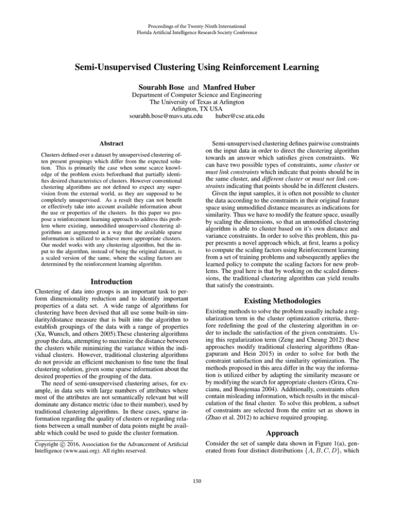
Consider the set of sample data shown in Figure 1(a), generated from four distinct distributions {A, B, C, D}, which
Existing Methodologies
Approach
150
(a) data from 4 distinct sources
(b) clusters formed before scaling
(c) clusters formed after scaling
Figure 1: (a): Original dataset and preferred final grouping; (b). Solution of traditional algorithm without dimension scaling;
(c). Solution of the same traditional algorithm with the X-axis scaled by a factor of 5
smaller number than the number of samples m. For example, given a set of 10 dimensional data of 100 points and
eight constraints, the resultant space after conversion would
be of 26 dimensions where the 10 features in the original
input are concatenated with the 16 new features computed,
where the similarity metric of the kernel is only computed
with respect to the points in the constraints.
Upon mapping the dataset onto the new feature space, the
new dimensions are scaled using a MDP (Markov Decision
Process) policy learned by the Reinforcement Learning algorithm and subsequently a traditional clustering algorithm
is applied on the new feature space, which now achieves the
desired clusters.
we want to divide into two clusters. Furthermore, an additional set of constraints are posed upon the dataset, which
provide evidence that the required clusters are the grouping
of sets {A, C} and {B, D} respectively. A clustering algorithm with Cartesian distance metric applied on the data,
groups the set of points into {A, B} and {C, D} as shown
in Figure 1(b). In order for the unmodified clustering algorithm to produce the desired result, the data is scaled up
along the x-axis by a factor of 5, thus increasing the distance
between two points along the x-axis while keeping the y-axis
variance the same. The clustering algorithm, in order to satisfy its own distance and variance optimization criteria, now
additionally satisfies the point constraints, achieving the desired grouping, as shown in Figure 1(c).
For a same cluster type constraint, the dimensions are to
be scaled in such a way that the points in the locality of
the constraint pair are closer in the new feature space. This
is achieved by shrinking the dimension along which they
are farthest apart. Similarly for a different cluster type constraints the dimensions along which they are closest are expanded, pushing them farther apart in the new feature space.
If the dimensions along which scaling is performed are
the same as those of the original inputs, the number and
forms of the potential final clusters are limited. For example, in a two dimensional scenario the final clusters formed
with two clusters can only be separated along the axes. In
order to address this problem this paper presents a novel approach where the original input dimension of the dataset is
appended to a kernel space with a similarity metric to each
pairwise point in the set of constraints. This provides the
scaling process with more degrees of freedom as it can scale
along a much higher number of dimensions, resulting in a
more complicated and nonlinear separation plane. Performing clustering in this reduced kernel space keeps the computational complexity lower compared to the complete kernel
space over all data points. A radial basis function (RBF) is
used as a kernel function (Zhang et al. 2007) since we need
our kernel function to have a local property where points
closer to each other should behave similarly. Thus, for input
data with m samples and d dimensions we convert the data
samples into a d + 2 ∗ c dimensional space where c is the
number of constraints, each specifying a pair of points over
which the constraint is defined. In general, this is a much
Similarity Function Learning
To apply Reinforcement Learning to the learning of the effective scaling of the feature dimensions, an MDP is defined.
An MDP (Puterman 1990), < S, A, T, R >, defines a
stochastic controllable process, where the state s ∈ S describes all information necessary to predict the transition
probabilities T : P (S |S, a) for every possible action a ∈ A.
Thus policies Π defining the actions to be taken only require
knowledge of the current state. The reward R : rQ(s, a)
defines the intermediate reward (payoff) obtained for taken
action a for a given state. The goal of solving an MDP is to
determine the policy Π(S, a) = P (a|S), that maximizes the
accumulated reward obtained. Reinforcement Learning is a
method to learn this policy.
In this work, the MDP uses two state variables, namely,
the accuracy for same cluster constraints and the accuracy
for different cluster constraints. Since the variables are continuous we discretize the state space into bins of size B. It
should be noted that, as with such discretizations, the choice
of discretization step is a trade-off between the fine grained
accuracy of the current state status and the computational
complexity.
State Space of the MDP
To compute state attributes, constraints are divided into two
groups, ones that are satisfied in the current clusters and ones
that are not. For the ones that are not satisfied, a degree of
them being satisfied is calculated. This degree is used as a
151
• For different cluster constraint type, fix unsatisfied constraint farthest from satisfaction
metric to identify how close to satisfied a constraint is. Using a probabilistic view on cluster membership, the probability of a point, x, being in a cluster, Ki , is defined as
• For different cluster constraint type, fix unsatisfied constraint closest to satisfaction
distance(x, Ki )
P (Ki |x) = j distance(x, Kj )
Upon choosing the specific constraint to fix, the dimensions
to scale are chosen. For same cluster constraint type, a subset of the dimensions with the highest distance is selected
and scaled down, bringing them closer in the new feature
space. Similarly for different cluster type, the dimensions
with the lowest distance are selected and scaled up, pushing
them farther apart.
The degree of a same cluster constraint, Cj,k , being satisfied
is a function of the probabilities of the two member points,
xj and xk , in the constraint. For each cluster, the likelihood
of them lying in the same cluster, Ki , is defined as
P (Ki |Cj,k , type(Cj,k ) = samecluster) =
P (Ki |xj ) ∗ P (Ki |xk )
Reward Function
and the degree of a same cluster type constraint to be fulfilled is then calculated as the maximum product of the probabilities for each point regarding every cluster. Thus the degree of a constraint being satisfied is the maximum likelihood for any class that both points are in that cluster. The
maximum (rather than the sum) is used here to achieve a
stronger tie across multiple constraints containing the same
data point since it forces a single cluster to be picked for
each constraint. Similarly, for a different cluster type constraint, Cj,k , the probability of a point belonging to cluster
Ki while the other does not, is defined as
The reward function is simply defined as the improvement
in the satisfaction of the constraints as measured by the sum
of the difference between each of the two accuracy variables
of the new state and the current state.
Goal State or End Criteria
The goal state is defined as the state where all the constraints
are satisfied. However it is often not possible to reach this
state due to many factors like human error in constraint selection or other contradicting constraints. Thus, in addition
to the above goal criteria we append another condition which
states that we end our search when the state does not change
for a given fixed number of steps.
P (Ki |Cj , k, type(Cj,k ) = dif f erentcluster) =
P (Ki |xj ) ∗ (1 − P (Ki |xk ))
and the degree of the constraint to be satisfied is again calculated as the maximum across all clusters of this probability.
The accuracy of a constraint type as a state variable is defined in Equation (1).
Pt (satisf ied) =
Experimental results
Problems for training, validation and testing were pseudorandomly generated as multivariate Gaussian distributions.
Parameters controlling the individual cluster size, number
of distinct clusters, mean and co-variance of each cluster,
along with the number of input dimensions were seeded randomly, with a range of 400 to 800 samples in each problem.
Furthermore, a set of constraints for each problem were randomly chosen from the data points. Reinforcement learning
was used to learn 5 different policies over a set of 70 training
problems. Subsequently, the policies were used to compute
the dimension scaling factors for 30 test problems similar to
their respective training problems which were unseen during
the policy learning phase.
For the experiments, a bin size of 0.05 was chosen, i.e.
state variable values are discretized into the accuracy intervals [0..0.05), [0.05..0.1), ..., [0.95..1]. For the actions,
scaling steps of 0.7 and 1.3 are chosen. For same cluster
constraints the top third of the dimensions with the highest distance are scaled down by multiplying the dimensions
by 0.7, and for different cluster constraints the bottom third
dimensions are scaled up by multiplying the selected dimensions by 1.3. The algorithms used were K-means clustering
(Hartigan and Wong 1979) for the clustering process and
SARSA(Rummery and Niranjan 1994) as the reinforcement
learning algorithm (Kaelbling, Littman, and Moore 1996)
for training the MDP. The policies were trained with problems similar to each other with respect to the number of
dimensions in the original dataset and the number of proposed constraints on the problem. Finally a policy was
#satisf ied constraints of type t
#constraints of type t
(1)
Accuracyt =
Pt (satisf ied) + (1 − Pt (satisf ied))∗ (2)
Ei∈unsatisf ied of type t [P (Ki |Cj,k , type(Cj,k ) = t)]
This results in two state attributes, Accuracysame cluster
and Accuracydif f erent cluster , which are both in the range
of [0..1]. We then discretize the attribute into bins of size B
in order to reduce the complexity since state values closer to
each other are related and thus can be grouped into a single
state, the size of the group determined by the bin size B.
Action Space of the MDP
Given the degrees of satisfaction of the individual constraints of any type, the unsatisfied constraints closest to
satisfaction and the constraints farthest from satisfaction are
identified, i.e. for each constraint type the unsatisfied constraints with the highest and the lowest probabilities are selected. There are 4 actions which the agent can take in every
state in order to satisfy the constraints.
• For same cluster constraint type, fix unsatisfied constraint
farthest from satisfaction
• For same cluster constraint type, fix unsatisfied constraint
closest to satisfaction
152
(a) Solutions for 2-dimensional dataset
(b) Solutions for 20-dimensional dataset mapped to 2
dimensions using t-sne for visualization
Figure 2: K-means clusters. (a). Solution without dimension scaling (Left); Solution with dimension scaling (Right) (b).
Solution of 20-dimensional data; Solution without dimension scaling (Left); Solution with dimension scaling (Right)
policy
1
2
3
4
5
# dimensions
2-7
5 - 10
7 - 15
15 - 20
2 - 20
# constraints
4 - 10
20 - 25
20 - 25
10 - 15
10 - 25
% satisfied
81.2%
84.8%
72%
73.33%
40%
References
Grira, N.; Crucianu, M.; and Boujemaa, N. 2004. Unsupervised and semi-supervised clustering: a brief survey. A
review of machine learning techniques for processing multimedia content, Report of the MUSCLE European Network
of Excellence (FP6).
Hartigan, J. A., and Wong, M. A. 1979. Algorithm as 136:
A k-means clustering algorithm. Journal of the Royal Statistical Society. Series C (Applied Statistics) 28(1):100–108.
Kaelbling, L. P.; Littman, M. L.; and Moore, A. W. 1996.
Reinforcement learning: A survey. Journal of artificial intelligence research 237–285.
Puterman, M. L. 1990. Markov decision processes.
Handbooks in operations research and management science
2:331–434.
Rangapuram, S. S., and Hein, M. 2015. Constrained 1spectral clustering. arXiv preprint arXiv:1505.06485.
Rummery, G. A., and Niranjan, M. 1994. On-line q-learning
using connectionist systems.
Van der Maaten, L., and Hinton, G. 2008. Visualizing data
using t-sne. Journal of Machine Learning Research 9(25792605):85.
Xu, R.; Wunsch, D.; et al. 2005. Survey of clustering algorithms. Neural Networks, IEEE Transactions on 16(3):645–
678.
Zeng, H., and Cheung, Y.-m. 2012. Semi-supervised
maximum margin clustering with pairwise constraints.
Knowledge and Data Engineering, IEEE Transactions on
24(5):926–939.
Zhang, J.; Marszałek, M.; Lazebnik, S.; and Schmid, C.
2007. Local features and kernels for classification of texture
and object categories: A comprehensive study. International
journal of computer vision 73(2):213–238.
Zhao, W.; He, Q.; Ma, H.; and Shi, Z. 2012. Effective semi-supervised document clustering via active learning
with instance-level constraints. Knowledge and information
systems 30(3):569–587.
Table 1: Performance analysis of individual policies
also trained with a broad range of problems, for comparison with the performance of the other specialized policies.
Figure 2 shows the result of a cluster output of K-means
on the original dataset and the output upon scaling the dimensions using the policies learned, red lines indicating different cluster type constraints while green lines indicating
same cluster type constraints. Figure 2(a) is a solution to a
2-dimensional problem using policy 1 while, Figure 2(b) is a
20-dimensional problem, the solution to which was mapped
to 2 dimensions using t-sne (Van der Maaten and Hinton
2008) for visualization. Table 1 shows the performance of
the individual policies on 30 test problems and the range of
dimensions and constraints learned upon. Policies 1 − 4 are
learned on specific types while policy 5 is a generic policy.
Since the constraints were randomly generated, it is often impossible to solve for all of them because of conflicting constraints. However, the solutions computed from the
policies above solve for the highest possible number of constraints while maximizing the accuracy of unsatisfied constraints as shown in Equation (2). Table 1 also shows that
policies learned for a specific type of problem (policies 1 to
4) perform much better than a generic policy (policy 5).
Conclusion
The paper shows that semi-unsupervised clustering is possible by re-mapping and scaling the original input dimensions, without modifying the clustering algorithm. Thus,
this method can be applied to any traditional clustering algorithm. This paper also shows that performance of generic is
poor compared to policies from specific types of problems.
153