The Workshops of the Thirtieth AAAI Conference on Artificial Intelligence
Artificial Intelligence for Smart Grids and Smart Buildings:
Technical Report WS-16-04
Identifying Contributing Factors of Occupant
Thermal Discomfort in a Smart Building
Aniruddha Basak,1 Ole Mengshoel,1 Stefan Hosein,2 Rodney Martin,3
Jayasudha Jayakumaran,1 Mario Gurrola Morga,4 and Ishwari Aghav1
Carnegie Mellon University Silicon Valley1 , University of the West Indies, St. Augustine2 ,
NASA Ames Research Center3 , Zapopan’s Superior Institute of Technology4
abasak@cmu.edu, ole.mengshoel@sv.cmu.edu, stefan.hosein2@my.uwi.edu,
rodney.martin@nasa.gov, jayasudha.jayakumaran@sv.cmu.edu,
mariogurrolam@gmail.com, ishwari.aghav@sv.cmu.edu
Abstract
Modeling occupant behavior in smart buildings to reduce energy usage in a more accurate fashion has garnered much recent attention in the literature. Predicting occupant comfort in
buildings is a related and challenging problem. In some smart
buildings, such as NASA AMES Sustainability Base, there
are discrepancies between occupants’ actual thermal discomfort and sensors based upon a weighted average of wet bulb,
dry bulb, and mean radiant temperature intended to characterize thermal comfort. In this paper we attempt to find other
contributing factors to occupant discomfort. For our experiment we use a dataset from a Building Automation System
(BAS) in NASA Sustainability Base. We choose one conference room for our experiment and empirically establish the
thermal discomfort level for the room’s temperature sensor.
We use various causality metrics and causal graphs to isolate candidate causes of the target room temperature. And we
compare these feature sets according to their predictive capability of future instances of discomfort. Moreover, we establish a trade off between computational and statistical performance of adverse event prediction.
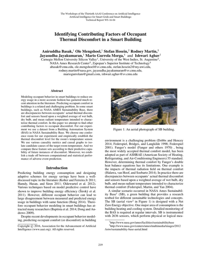
Figure 1: An aerial photograph of SB building.
environment is a challenging problem (Dobbs and Hencey
2014; Federspiel, Bridges, and Langkilde 1998; Federspiel
2001). Fanger’s model (Fanger and others 1970) , being
the most widely accepted thermal comfort model, has been
adopted as part of ASHRAE (American Society of Heating,
Refrigerating, and Air-Conditioning Engineers) 55 standard.
However, determining thermal comfort by Fanger’s double
heat balance equations has its limitations. One example is
the impacts of thermal radiation field on thermal comfort
(Halawa, van Hoof, and Soebarto 2014). In practice there are
discrepancies between occupants’ actual thermal discomfort
and sensors based upon a weighted average of wet bulb, dry
bulb, and mean radiant temperature intended to characterize
thermal comfort (Federspiel, Martin, and Yan 2004).
A similar scenario occurred in NASA Ames Sustainability Base1 (SB), a green building that provides a research
testbed for different sustainable technologies and concepts.
The SB (aerial view2 in Figure 1) is designed with a Net
Zero Energy objective. One major area of consumption is the
building heating and cooling system. Detailed monitoring of
the BAS is required at regular intervals. SB is instrumented
with 2636 sensors, which perform physical or logical mea-
Introduction
Predicting building energy consumption and designing
adaptive schemes for energy savings have been a welldiscussed topic in the literature (Kolter and Ferreira Jr 2011;
Hamdy, Hasan, and Siren 2011; Oldewurtel et al. 2012).
Various techniques based on model predictive control have
shown to improve building energy efficiency (Širokỳ et al.
2011). However, different occupant behavior can lead to
large disagreement between measured and predicted energy
usage in buildings with same function (Hong 2014). Therefore occupant behavior modeling in smart buildings has attracted many researchers (Baptista et al. 2014; Dong and Andrews 2009).
Despite recent developments in occupant behavior modeling, predicting occupant comfort (or discomfort) in building
1
http://www.nasa.gov/ames/facilities/sustainabilitybase
http://www.nasa.gov/centers/ames/multimedia/images/2012
/iotw/sustainability-base-aerial.html
2
c 2016, Association for the Advancement of Artificial
Copyright Intelligence (www.aaai.org). All rights reserved.
219
False alarm rate


 x1 x2 · · · xp 
Causal
subsets
isolating
Adverse
event
prediction
Missed detection rate
Detection time
Figure 2: Data processing steps
ods have also been applied for thermal comfort forecasting. Locally weighted regression has been shown to provide
more accurate prediction than PMV in (Manna, Wilson, and
Brown 2013). To the best of our knowledge, causal learning
algorithms have not been used to identify the contributing
factors to thermal comfort.
surements. From Nov 2014 to May 2015 many “cold complaints” were issued by the occupants. A cold complaint can
originate from an anomalous drop in building temperature
or unexpected cool environment in conference rooms in the
morning.
An essential step to eliminating these complaints is to
identify the contributing factors to occupant discomfort. In
this work we use a few causal discovery methods to solve
this problem in a data driven approach. First, we established
an empirical threshold of a conference-room’s temperature
for representing the associated cold complaints. We call this
room temperature sensor, the “target variable” (x∗ ). Next we
used the sensor data collected from the BAS of the SB building to learn causal subsets relevant to that temperature sensor. Autoregressive model, Granger causality test and causal
graphs were used as learning models in the experiments.
The causal subsets were then fed to an adverse event prediction toolbox, ACCEPT (Adverse Condition and Critical
Event Prediction Toolbox) (Martin et al. 2015), which provides a single, unifying framework for comparative performance assessment of results from the application of a variety of algorithmic methods. ACCEPT produces results in the
form of missed detection (false negative), false alarm (false
positive) rate and detection time (the number of time steps in
advance the system can predict an anomalous event), which
are essential in generating our results.
Procedure
The data processing components of our analysis is shown
in Figure 2. Using multiple causal learning techniques we
isolated subsets of features from time series data collected
from the BAS. These feature subsets are used for adverse
event prediction. The performance metrics of prediction are
false alarm rate (false positive rate), missed detection rate
(false negative rate) and the detection time (the number of
timesteps in advance a warning is generated).
In this section we describe the casual isolation methods
and adverse event prediction technique.
Causal subsets isolation
• Granger Causality test, a hypothesis test promoted by
the econometrician Clive Granger (Granger 1969), helps
in determining whether the past values of one time series
can be leveraged in predicting the future values of another.
Hence, this test can be directly used to identify features
with causal relationship with the target (x∗ ).
This causality test is based on a series of F-tests where
each test determines if a feature has statistically significant information about the future values of x∗ . The test
statistic has a F-distribution under the null hypothesis.
For each variable xi , the null and alternative hypothesis
for the test are as follows
Related Research
A comprehensive overview of many methods to evaluate and predict occupant thermal comfort is presented in
(Olesen 2004; Federspiel, Bridges, and Langkilde 1998).
Lately, various machine learning techniques have been applied to model thermal comfort. Different human body factors (blood volume pressure, skin temperature, respiration
rate and skin conductance) and environmental measurements (e.g ambient temperature, humidity, air motion and so
forth) have been used to prediction occupant comfort levels
using correlations and Predictive Mean Vote (PMV) model
(Burzo et al. ). The impact of climate, glazing type, and
shading properties on thermal comfort in an office environment has been studied in (Bessoudo et al. 2010).
Identifying the more suitable set of features among environmental, psychological and physiological attributes, to
predict thermal comfort level, have also been attempted
(Farhan et al. 2015). The authors compared Support Vector Machine (SVM) and Random Forest classifiers with
Fanger’s model and found that the accuracy of SVM classifier was two times higher than Fanger’s model. Kernel meth-
H0 : xi does not Granger cause x∗
H1 : xi Granger causes x∗ .
The linear model according to H1 is called unrestricted
(U R) regression model. And the model without xi , as
per H0 , serves as the restricted (R) regression model. The
parameters of these models are learned form the training
data. If the sum of squared residuals of the trained R and
U R models are SSRR and SSRU R respectively, the test
statistic (F ) is defined as follows,
F =
(SSRR − SSRU R )/p
(SSRU R )/(N − p − 1)
(1)
where N is the number of observations in training data
and p is the number of variables.
220
If the value of F is greater than the critical value of Fdistribution, the null hypothesis is rejected. This critical
value is dependent on the significance level (α) of the test.
If the null hypothesis is rejected for xi , it is considered to
Granger cause x∗ .
• Autoregressive (AR) models are often used in economics and for modeling time-varying natural processes
(Kelejian and Prucha 2010; Chakraborty et al. 2012). We
used an autoregressive model of order τ , AR(τ ), to express the target as a linear combination of all time-lagged
variables,
(j)
yt
(j)
= aT1 yt−1 + aT2 yt−2 + · · · + aTτ yt−τ + et
T
= β Yt−1,t−τ +
(2)
(j)
et
Figure 3: Architecture of ACCEPT.
(j)
where yt = x∗ is the target, yt ∈ Rp is a vector containing the values of all variables at time t and at is the corresponding weight vector. Yt−1,t−τ ∈ Rpτ and β ∈ Rpτ
concatenates the variables and weights respectively. To reduce non-informative variables we train the model with
a sparsity constraint. Our optimization formulation is as
follows,
T
X
2
(j)
β̂L = arg min
yt − Yt−1,t−τ β + λ||β||L (3)
β∈Rpτ
Adverse Event Prediction
Adverse event prediction is the process of identifying potential adverse events in a system before they occur. This
is necessary for situations where an adverse event can be
problematic or fatal. By selecting informative features, prediction can occur within a reasonable time horizon of an
actual adverse event so that mitigating action can be taken
to stop the adverse event from occurring. Hence, we use the
ACCEPT (Adverse Condition and Critical Event Prediction)
Toolbox (Martin et al. 2015) to perform this prediction.
In ACCEPT, all data is preprocessed and filtered. In
Fig. 3, the regression toolbox contains multiple regression
techniques as support vector regression (SVR), k-nearest
neighbor regression (k-NN), linear regression (LR), bagged
neural nets (BNN), extreme learning machines (ELM), etc.
We use LR and ELM in our experiments. ELM is similar to
a single layer feed-forward neural network with one difference that the input layer parameters are assigned randomly.
ACCEPT employs an unsupervised machine learning approach for its architecture, meaning that no labeled data is
used to supervise the process of model learning. As such,
all training data associated with the regression step is by
definition nominal data. Anomalous data is reserved solely
for validation and testing purposes, and does not influence
the model characterized by the regression step described
above. In this way, two distinct classes of machine learning algorithms, regression and classification, are employed
within ACCEPT. Classification methods based upon hypothesis tests are used to determine if any novel, anomalous data
is out of family with respect to the regression model characterizing the nominal training data.
The results of ACCEPT contain the false alarm rate, the
missed detection rate and the detection time. Here, the detection time is defined as the number of timesteps in advance
a warning is generated. By utilizing these metrics we can
compare the different causal learning techniques.
t=τ
where the regularization norm, L, is chosen to 2. We select the first k variables, sorted in decreasing order of the
weights in the trained model β̂L , as informative variables.
• Causal graph learning We use two causal graph structure learning algorithms: PC and GES. Both are widely
used methods and theoretically correct.
PC (Spirtes and Glymour, Social Science Computer Review, 1991) is a pattern search algorithm for which the input
is an acyclic causal structure. The input dataset should be
either entirely continuous or entirely discrete. When the input dataset is continuous, the causal relation between any
two variables is linear and the distribution for each variable
is Normal. The PC algorithm sometimes outputs doubleheaded edges on a large sample limit. This indicates that
the adjacent variables have an unrecorded common cause.
PC algorithm constructs the graph structure based on conditional independence relations in the data. For continuous
datasets, PC algorithm uses tests of zero correlation or zero
partial correlation for independence or conditional independence respectively.
The GES algorithm is a stable greedy equivalency search
algorithm that runs under the same input assumptions as the
PC algorithm but the output patterns are always the same.
The GES is a score based algorithm. It scores all possible orientations of edges between variables, and higher the
score, the better the approximation should be. The penalty
discount, the parameter given to the GES algorithm affects
which edges are discarded. The higher the penalty discount
the more robust an edge must be to remain the output graph.
One variation of the GES algorithm is the iMAGES algorithm which runs the GES algorithm on all datasets multiple
times, with increasing penalty discounts, until there are no
three-variable cliques left in the graph.
Experiments and Results
Data and Methods
Our data set consists 26,493 samples (Nov 2014 to Feb
2015) from 2,636 sensors of the BAS of NASA SB building.
221
Type of Sensor
Temperature
Current
Valve
Set point
Others
Number of sensors
273
191
201
267
581
Table 1: Feature categories in the NASA SB dataset
These sensors measure various physical and logical quantities (such as room temperature, humidity, pressure in flow
pipes, status of heat pump, etc) and record in 5 minutes interval. A brief categorical description of the features is presented in Table 1.
As a preprocessing step of our experiments, we centered
and scaled every sensor data to make the mean 0 and variance 1. We used 60% of total samples for training models,
10% for validation and 30% for testing.
While training autoregressive model, we observed that
strong correlations exist among room-temperature sensors
measurements. As temperature in different rooms is controlled by a central heating-cooling system, similar variations exist in multiple room-temperature sensors. Thus for
proper causal discovery, we removed all temperature sensors, except the target, from the dataset.
In the first set of experiments we isolate the causal subsets
using the previously described methods. A summary of all
subsets is presented in Table 2. Next we establish an empirical comfort threshold for the target variable. Finally we use
ACCEPT to compare the predictability of the causal subsets
in forecasting adverse events of the target variable.
Figure 4: Cold and warm temperature regions according to
empirical analysis.
• Causal graph learning We use PC and GES algorithms
to learn causal graph over the variables in the dataset.
As the computation time of structure learning with large
number of features is very high (Figure 8), we attempted
to learn causal variables with all features and a subset of
informative variables. For the first case, we denote the
full
identified causes as CPC/GES
. And the causes identified
from a graph learned over k informative variables are dek
noted by CPC/GES
.
For the PC algorithm, we used Gaussian conditional independence test with significance level α = 0.01. And
the score function for GES algorithm was Bayesian Information Criterion (BIC). We found that the graph structure
changes significantly with increasing number of features
fed to the structure learning algorithm. Thus the set of
identified causes does not always grow with increasing
features, i.e
Causal subsets isolation
• GC test Using significance level α = 0.005, we perform
the F-tests for every feature in the dataset. We construct a
causal subset by including all features in GCtest for which
the null hypothesis was rejected.
Moreover, we sort the features in GCtest according to their
deviation from the critical value of F-test and choose the
top features as candidate causes. The subset with top k
k
.
features is denoted as GCtest
k1
k2
full
CPC
* CPC
* CPC
for any k1 < k2 < p.
(4)
Empirical discomfort threshold
An empirical approach was taken to determine the ground
truth for the cold complaints prediction scenario. We estimated the distribution of the target room temperature
sensor (x∗ ) and found that it was a unimodal distribution with mean 71.7 and standard deviation 1.8. Hence,
a 95% confidence interval around the mean corresponds
to 68.1◦ F and 75.3◦ F. Considering this range as nominal room temperature values, we established 68.1◦ F as
the upper threshold for cold regions. In our problem, we
are only concerned with anomalous drops in temperature.
Thus, we considered any temperature value below 68.1◦ F
as an adverse event (cold). And there are multiple adverse
events as shown in Figure 4.
• Autoregressive model training First, we train an AR(1)
model with x∗ as output and all sensors in the dataset as
inputs. Due to rank deficiency of the training data matrix, we add a small ridge penalty (λ) on the parameters.
We compare this model with an AR(1) model trained with
tuned λ. The tuning is performed in a separate validation
set.
Figure shows the predictions of these two models. Clearly,
the trained model with tuned λ shows superior performance than the small λ counterpart. We use the model parameters of the tuned to select informative variables from
the dataset. As all features are in the same scale (part of
pre-processing), we select k informative variables as the
top k features, sorted in descending order of the parameter
k
values. The denote this set as CAR+ridge
.
Comparison using ACCEPT
The goal of this experiment is to compare the performance
of causal subsets in predicting adverse events of the target
based on the derived empirical threshold. As ACCEPT is
222
Feature Set (F )
5
10
20
GCtest
, GCtest
, GCtest
5
CAR+ridge
,
10
CAR+ridge
,
20
CAR+ridge
,
100
CAR+ridge
Number of
features |F |
5, 10, 20
5,
10,
20,
100
Identification
method
Granger
causality
test
AR model
with ridge
penalty
5
10
20
CGES
, CGES
CGES
3, 1, 6
GES algorithm
5
CPC
,
3, 1, 6
PC algorithm
10
CPC
,
20
CPC
p/2
100
full
CPC
, CPC , CPC
False
Alarm
Rate (%)
Missed
Detection
Rate (%)
Detection
Time
(minutes)
5
GCtest
24.20
0.00
102.50
10
GCtest
24.20
0.00
102.50
20
GCtest
24.20
0.00
102.50
5
CAR+ridge
10
CAR+ridge
20
CAR+ridge
100
CAR+ridge
5
CGES
10
CGES
20
CGES
5
CPC
10
CPC
20
CPC
100
CPC
p/2
CPC
full
CPC
22.00
0.00
97.50
21.00
0.00
97.50
21.55
0.00
97.50
13.38
1.90
100.00
25.27
0.00
102.50
2.44
0.48
100.00
7.86
0.00
102.50
8.28
0.00
52.50
8.28
0.00
52.50
5.20
0.00
52.50
14.54
0.95
97.50
23.25
0.00
100.00
23.14
0.00
100.00
Feature
Set
6, 7, 6
Table 2: Descriptions of all feature set
Table 3: Results for all causal subsets
discrete features are discarded from each causal subset.
First we compare the linear regression (LR) and extreme
learning machine (ELM) models, as part of ACCEPT’s regression toolbox, in terms of false alarm rates and detection
times. Missed detection rates are very small in all cases and
thus omitted. Figure 5 shows the comparison prediction results for one feature set from each identification method. We
observe that in all cases, ELM model performs similar or
better than LR model. Hence, for the next experiments we
exclusively use ELM model for regression in ACCEPT.
Table 3 shows the results for all causal subsets produced
by ACCEPT. There is no subset which achieves minimum
false alarm and missed detection rates which maximizing the
detection time. To comprehend the results we first compare
the subsets form each identification method separately. Then
we make inter-method comparison.
Figure 6 shows results of AR model features with increasing feature set sizes. We see an inverse relation between
false alarm rate and detection time. Moreover, with small
100
increase in detection time CAR+ridge
achieves significant decrease in false alarm rate. Hence we can conclude that the
causal subsets (of AR model) with higher size have superior
predictability of adverse events.
(a) Comparison of false alarm rates.
(b) Comparison of detection times.
Figure 5: Comparison of Extreme Learning Machine (ELM)
and Linear Regression (LR) models.
|F |
There is no change in prediction performance of GCtest
|F |
subsets with increasing size (Table 3). However CAR+ridge
designed to train models only using continuous features, the
223
|F |
Figure 6: Comparison of ACCEPT results for CAR+ridge features.
Figure 8: Runtime comparison of causal subset identification (PC and AR) and adverse event prediction combined,
with increasing number of features.
inated by ACCEPT’s run-time.
On the contrary, causal subsets isolated by the PC algorithm do not grow with increasing features in the dataset.
Thus the computational cost, in this case, is dominated by
PC run-time. Figure 8 compares the run-times of causal subset identification and adverse event prediction combined, for
increasing feature set sizes. In both ACCEPT performs prediction. We observe that both grow super-linearly. However
the run-time of “AR + ACCEPT” is a few-order magnitude
higher than the “PC + ACCEPT”. Although AR model’s
causal features exhibit more stable statistical performance,
they demand much higher computational time. Thus we can
conclude that a good trade-off between computational and
statistical performance can be achieved using the PC algorithm.
Figure 7: Comparison of ACCEPT results for causal features
identified by the PC algorithm.
Conclusion and Future Work
|F |
achieves lower false alarm rate than GCtest with approximately similar detection time. Hence the AR model in superior to Granger causality test for this problem.
k
Small variation in the false alarm rates is seen for CGES
subsets. In contrast significant variations in all three metrics
k
can be observed for CPC
features. Figure 7 compares the performance of these causal subsets. The best trade-off between
20
the three metrics is accomplished by CPC
.
k
Although CPC subsets do not grow monotonically with
increasing k, we observed that there are one or many overlapping features among all subsets. This indicate high significance of these overlapping features in affecting thermal
discomfort.
In this work we presented an alternate approach for identifying contributing factors of occupant discomfort. We used
various causal learning method to isolate candidate causes
associated with a target room-temperature. Empirically, we
established the discomfort level for a conference room and
used the candidate causes to predict cold temperatures in the
room. We found that the candidate causes identified by autoregressive model and the PC algorithm explained the adverse events well. However, good trade off between computation time and prediction accuracy was achieved by the
PC algorithm. Thus we recommend causal graph learning
approach for occupant discomfort modeling.
Future work will be directed towards using the discomfort
model to design energy efficient schemes for maintaining
occupant comfort in smart buildings.
Trade-off between computational and statistical
performance
We observed that the training time in ACCEPT increases
non-linearly with increasing number of features. In the previous comparison we observed superior performance from
causal subsets identified by AR model and the PC algorithm.
Also we seen large feature sets are required for low false
alarm rate by AR model subsets. Here the computational
cost of adverse event prediction using these subsets is dom-
References
Baptista, M.; Fang, A.; Prendinger, H.; Prada, R.; and Yamaguchi, Y. 2014. Accurate household occupant behavior
modeling based on data mining techniques. In Proceedings
of the Twenty-Eighth AAAI Conference on Artificial Intelligence, 1164–1170.
224
sive and heteroskedastic disturbances. Journal of Econometrics 157(1):53–67.
Kolter, J. Z., and Ferreira Jr, J. 2011. A large-scale study on
predicting and contextualizing building energy usage.
Manna, C.; Wilson, N.; and Brown, K. N. 2013. Personalized thermal comfort forecasting for smart buildings via
locally weighted regression with adaptive bandwidth. In
SMARTGREENS, 32–40.
Martin, R.; Das, S.; Janakiraman, V.; and Hosein, S. 2015.
ACCEPT: Introduction of the adverse condition and critical event prediction toolbox. Technical Report NASA/TM2015-218927, National Aeronautics and Space Administration (NASA).
Oldewurtel, F.; Parisio, A.; Jones, C. N.; Gyalistras, D.; Gwerder, M.; Stauch, V.; Lehmann, B.; and Morari, M. 2012.
Use of model predictive control and weather forecasts for
energy efficient building climate control. Energy and Buildings 45:15–27.
Olesen, B. W. 2004. International standards for the indoor
environment. Indoor Air 14(s7):18–26.
Širokỳ, J.; Oldewurtel, F.; Cigler, J.; and Prı́vara, S. 2011.
Experimental analysis of model predictive control for an
energy efficient building heating system. Applied Energy
88(9):3079–3087.
Bessoudo, M.; Tzempelikos, A.; Athienitis, A.; and Zmeureanu, R. 2010. Indoor thermal environmental conditions
near glazed facades with shading devices–part i: Experiments and building thermal model. Building and Environment 45(11):2506–2516.
Burzo, M.; Wicaksono, C.; Abouelenien, M.; Pérez-Rosas,
V.; Mihalcea, R.; and Tao, Y. Multimodal sensing of thermal
discomfort for adaptive energy saving in buildings.
Chakraborty, P.; Marwah, M.; Arlitt, M. F.; and Ramakrishnan, N. 2012. Fine-grained photovoltaic output prediction
using a bayesian ensemble. In AAAI Conference on Artificial
Intelligence.
Dobbs, J. R., and Hencey, B. M. 2014. Model predictive hvac control with online occupancy model. Energy and
Buildings 82:675–684.
Dong, B., and Andrews, B. 2009. Sensor-based occupancy
behavioral pattern recognition for energy and comfort management in intelligent buildings. In Proceedings of building
simulation, 1444–1451.
Fanger, P. O., et al. 1970. Thermal comfort. analysis and applications in environmental engineering. Thermal comfort.
Analysis and applications in environmental engineering.
Farhan, A. A.; Pattipati, K.; Wang, B.; and Luh, P. 2015.
Predicting individual thermal comfort using machine learning algorithms. In Automation Science and Engineering
(CASE), 2015 IEEE International Conference on, 708–713.
IEEE.
Federspiel, C. C.; Bridges, B.; and Langkilde, G. 1998. Statistical analysis of unsolicited thermal sensation complaints
in commercial buildings/discussion. ASHRAE Transactions
104:912.
Federspiel, C. C.; Martin, R. A.; and Yan, H. 2004. Recalibration of the complaint prediction model. HVAC&R Research 10(2):179–200.
Federspiel, C. 2001. Estimating the frequency and cost of
responding to building complaints in: Spengler, j. sammet
j. and mccarthy, j. eds. Indoor Air Quality Handbook, McGraw Hill.
Granger, C. W. 1969. Investigating causal relations by
econometric models and cross-spectral methods. Econometrica: Journal of the Econometric Society 424–438.
Halawa, E.; van Hoof, J.; and Soebarto, V. 2014. The impacts of the thermal radiation field on thermal comfort, energy consumption and controla critical overview. Renewable
and Sustainable Energy Reviews 37:907–918.
Hamdy, M.; Hasan, A.; and Siren, K. 2011. Impact of
adaptive thermal comfort criteria on building energy use and
cooling equipment size using a multi-objective optimization
scheme. Energy and Buildings 43(9):2055–2067.
Hong, T. 2014. Occupant behavior: impact on energy use
of private offices. In ASim 2012-1st Asia conference of International Building Performance Simulation Association.,
Shanghai, China, 11/25/12-11/27/12.
Kelejian, H. H., and Prucha, I. R. 2010. Specification and
estimation of spatial autoregressive models with autoregres-
225