Proceedings of the Ninth Symposium on Abstraction, Reformulation and Approximation
Classifying Scientific Publications Using Abstract Features
Cornelia Caragea1 , Adrian Silvescu2 , Saurabh Kataria1 , Doina Caragea3 , and Prasenjit Mitra1
1
Information Sciences and Technology, Pennsylvania State University
2
Naviance Inc., Oakland, CA
3
Computer and Information Sciences, Kansas State University
{ccaragea,skataria,pmitra}@ist.psu.edu
silvescu@gmail.com, dcaragea@ksu.edu
Abstract
learning algorithms
With the exponential increase in the number of documents available online, e.g., news articles, weblogs,
scientific documents, effective and efficient classification methods are required in order to deliver the appropriate information to specific users or groups. The
performance of document classifiers critically depends,
among other things, on the choice of the feature representation. The commonly used “bag of words” representation can result in a large number of features. Feature abstraction helps reduce a classifier input size by
learning an abstraction hierarchy over the set of words.
A cut through the hierarchy specifies a compressed
model, where the nodes on the cut represent abstract
features. In this paper, we compare feature abstraction
with two other methods for dimensionality reduction,
i.e., feature selection and Latent Dirichlet Allocation
(LDA). Experimental results on two data sets of scientific publications show that classifiers trained using
abstract features significantly outperform those trained
using features that have the highest average mutual information with the class, and those trained using the
topic distribution and topic words output by LDA. Furthermore, we propose an approach to automatic identification of a cut in order to trade off the complexity of classifiers against their performance. Our results
demonstrate the feasibility of the proposed approach.
SVM,NB
SVM
NB
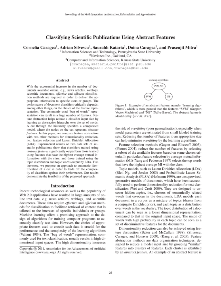
Figure 1: Example of an abstract feature, namely “learning algorithms”, which is more general than the features “SVM” (Support
Vector Machines) and “NB” (Naı̈ve Bayes). The abstract feature is
identified by {SV M, N B}.
the risk of overfitting (poor generalization), especially when
model parameters are estimated from small labeled training
sets. Reducing the number of features to an appropriate size
can help minimize overfitting by the learning algorithms.
Feature selection methods (Guyon and Elisseeff 2003),
(Fleuret 2004), reduce the number of features by selecting
a subset of the available features based on some chosen criteria. In particular, feature selection by average mutual information (MI) (Yang and Pederson 1997) selects the top words
that have the highest average MI with the class.
Topic models, such as Latent Dirichlet Allocation (LDA)
(Blei, Ng, and Jordan 2003) and Probabilistic Latent Semantic Analysis (PLSA) (Hofmann 1999), are unsupervised,
generative models of documents, which have been successfully used to perform dimensionality reduction for text classification (Wei and Croft 2009). They are designed to uncover hidden topics, i.e., clusters of semantically related
words that co-occur in the documents. LDA models each
document in a corpus as a mixture of topics (drawn from
a conjugate Dirichlet prior), and each topic as a distribution
over words in the vocabulary. The topic distribution of a document can be seen as a lower dimensional representation,
compared to that in the original input space. The union of
words with high probability in each topic can be seen as a
set of discriminative features for the documents.
Dimensionality reduction can also be achieved using feature abstraction (Baker and McCallum 1998), (Silvescu,
Caragea, and Honavar 2009), (Kang et al. 2005). Feature
abstraction methods are data organization techniques, designed to reduce a model input size by grouping “similar”
features into clusters of features. Each cluster is identified
by an abstract feature. An example of an abstract feature is
Introduction
Recent technological advances as well as the popularity of
Web 2.0 applications have resulted in large amounts of online text data, e.g. news articles, weblogs, and scientific
documents. These data require effective and efficient methods for classification to facilitate retrieval of content that is
tailored to the interests of specific individuals or groups.
Machine learning offers a promising approach to the design of algorithms for training computer programs to accurately classify text data. However, the choice of appropriate features used to encode such data is crucial for the
performance and the complexity of the learning algorithms
(Valiant 1984). The “bag of words” representation, commonly used for text classification, usually results in high dimensional input spaces. The high dimensionality increases
c 2011, Association for the Advancement of Artificial
Copyright Intelligence (www.aaai.org). All rights reserved.
26
Pereira, and Bialek 1999), (Slonim and Tishby 1999),
(Pereira, Tishby, and Lee 1993) are distributional clustering based approaches, designed to find a compression of a
variable X while preserving as much information as possible about a target (or relevance) variable Y . Baker and
McCallum (1998) applied distributional clustering (Pereira,
Tishby, and Lee 1993) to reduce the dimensionality of the
feature space for document classification tasks. They compared the distributional clustering based approach with the
Latent Semantic Indexing (Deerwester et al. 1990), and feature selection (Yang and Pederson 1997), and found that
their approach can significantly reduce a model input size
for a small decrease in the accuracy of the “bag of words”
models. Slonim and Tishby (2001) compared feature abstraction by bottom-up agglomerative IB with feature selection on text documents, whereas Bekkerman et al. (2003)
compared feature abstraction by top-down IB with feature
selection on binary and multi-label text classification tasks.
Both studies found that using feature abstraction yields significant improvement in classification performance over the
“bag of words” models. Unlike the above works, we compare the (bottom-up) feature abstraction with LDA on multiclass text documents, in addition to feature selection.
Depending upon the application needs, the basic LDA
framework (Blei, Ng, and Jordan 2003) has been extended
by various research efforts. For example, the “bag of word”
assumption in LDA is relaxed to the “bag of n-grams” such
that the topics are distributions over n-grams (Wang and
McCallum 2005). DiscLDA (Lacoste-Julien, Sha, and Jordan 2009) is a variant of LDA aimed at finding useful lowdimensional document representations, but also taking into
account class label information in deriving these representations, i.e. DiscLDA is a supervised variant of the unsupervised LDA. Hierarchical Topic Models (Blei et al. 2004) aim
at organizing the hidden topics in the data into a hierarchy.
In this study, we compare feature abstraction (under the “bag
of words” assumption) with “vanilla” LDA; a comparison
among the other methods will be pursued in the future.
desJardins, Getoor, and Koller (2000) explored the use
of abstraction-based search to compress conditional probability tables in Bayesian networks. Furthermore, Kang et
al. (2005) automatically constructed word taxonomies from
text data and used Minimum Description Length (Mitchell
1997) to search for a “good” cut through the word taxonomy.
For a given cut, the authors explored the expansion of each
node on the cut. In contrast, we use Akaike and Bayesian
Information Criteria, and explore the cuts in a predefined order, specifically the order in which the nodes were added to
the abstraction hierarchy, hence, making the procedure more
efficient than that of Kang et al. (2005).
shown in Figure 1. Feature abstraction effectively reduces
the number of parameters of standard model by one to three
orders of magnitude without sacrificing classification accuracy (Baker and McCallum 1998), (Silvescu, Caragea, and
Honavar 2009). Specifically, it learns an abstraction hierarchy over the set of features using hierarchical agglomerative clustering (Duda, Hart, and Stork 2001), based on the
Jensen-Shannon divergence (Lin 1991). A cut or level of abstraction through the resulting abstraction hierarchy specifies a compressed model, where the nodes on the cut are used
as “features” in the classification model. Abstraction acts
as a regularizer that helps minimize overfitting (through parameter smoothing) when the training set is limited in size,
i.e., it improves the statistical estimates of complex models
by reducing the number of parameters, and hence, can yield
more accurate models compared to “bag of words” models.
In this paper, we address two main questions. The first
question is: how does feature abstraction compare with two
other dimensionality reduction methods, i.e., feature selection by average MI and LDA? We compare feature abstraction as described in (Silvescu, Caragea, and Honavar 2009)
with feature selection by average MI (Yang and Pederson
1997) and LDA (Blei, Ng, and Jordan 2003) on scientific
document classification. Given that both feature abstraction and LDA identify clusters of words in documents, i.e.,
abstractions and topics, respectively, we analyze the interpretability of the resulting abstractions by directly comparing them with the topics produced by LDA.
The second question that we address is how to identify a
“good” cut automatically through an abstraction hierarchy,
i.e., a cut which results in simple and accurate classifiers?
We extend the work of (Silvescu, Caragea, and Honavar
2009) to address its shortcomings. Specifically, we propose
the use of a scoring function to search for a “good” cut,
in a greedy, top-down fashion, to trade off the complexity
of a classifier against its performance. To penalize complex
classifiers, we evaluate two different “information criteria”,
namely the Akaike Information Criterion (Akaike 1974) and
the Bayesian Information Criterion (Schwarz 1978). Note
that the procedure does not necessarily find the optimal cut
through the abstraction hierarchy, however, we experimentally show that we obtain a “good” trade-off between the
complexity and the accuracy of the classifiers.
The results of our experiments on two data sets of scientific publications show that: (i) feature abstraction can yield
significantly more accurate models than those trained using
the “bag of words”, those trained using features that have
the highest average MI with the class, and those trained using the topic distribution and topic words output by LDA
(for example, the abstraction-based classifiers show 25%43% error reduction over the “bag of words” models); (ii)
the proposed scoring functions are capable of identifying a
“good” cut, which can produce classifiers that use significantly smaller number of features and, at the same time, are
more accurate than those using the “bag of words” approach.
Feature Representations
We describe three dimensionality reduction methods for text
classification: one based on feature selection by average
mutual information (Yang and Pederson 1997), one based
on topic models (Blei, Ng, and Jordan 2003), and another
one based on the feature abstraction approach of (Silvescu,
Caragea, and Honavar 2009). In what follows, we denote by
D = {(wl , cl )}l=1,···,N a data set of documents wl and their
Related Work
In this section, we discuss the most relevant works to our
study. Information Bottleneck (IB) and its variants (Tishby,
27
associated class labels cl ; by V the set of words of size n; and
by m the desired reduced space dimensionality (m n).
Feature Abstraction
Feature abstraction reduces a classifier input size by finding
clusters of “similar” features, called abstract features.
Constructing abstract features. The algorithm for constructing abstract features (or abstractions) is based on hierarchical agglomerative clustering (Duda, Hart, and Stork
2001). The input is a data set D = {(wl , cl )}l=1,···,N of
text documents wl and their class labels cl . The output is
an abstraction hierarchy T over the set of words V of size
n, extracted from D. An abstraction hierarchy (AH) over
V is defined as a rooted tree such that the leaf nodes correspond to the words in V and the internal nodes correspond
to abstractions or clusters of words. An m-cut γm through
T is a set of m nodes, which forms a partition of V, i.e.,
γm = {a1 : V1 , · · · , am : Vm }, where ai denotes the ith
abstraction and Vi denotes the subset of words that are clustered together into ai based on some similarity measure.
The algorithm initializes each abstraction ai with a word
wi in V, and recursively merges pairs of abstractions that are
most “similar” to each other. The AH T , which is stored in
a last-in-first-out (LIFO) stack, is returned after n − 1 steps.
Note that T is constructed in a bottom-up fashion.
Two abstractions are considered to be “similar” if they occur within similar class contexts. The class context of a word
wi in V is defined as the conditional probability distribution
p(C|wi ) of the class variable C given the word wi , which is
estimated from D as follows:
#[wi , cj ]
,
(2)
p̂(C|wi ) = cj ∈C #[wi , cj ]
Feature Selection
Feature selection is performed by selecting a subset F of
features (i.e., words) from V, F ⊆ V such that |F| = m.
The features are ranked according to a scoring function f
and the top m best ranked features are selected.
As the scoring function, we used the average mutual information (Cover and Thomas 1991) between the class variable, denoted by C, which takes values in the set of the available classes C, and the random variable over the absence or
presence of a word wi in a document, denoted by Wi , which
takes values 0 or 1, respectively. The average mutual information is defined as follows:
I(C, Wi )
=
=
H(C) − H(C|Wi )
(1)
p(C, Wi )
p(C, Wi ) log
p(C)p(Wi )
C∈C Wi ∈{0,1}
where H(C) is the entropy of the class variable, and
H(C|Wi ) is the entropy of the class variable conditioned
on the absence or presence of word wi . The probability
p(C, Wi ) is estimated from counts gathered from D and
p(C) and p(Wi ) are obtained by marginalizing p(C, Wi ).
The feature selection representation. Let (wl , cl ) be an
instance in D. The “bag of words” representation of (wl , cl )
is given by: ([w1 : #w1l ], · · · , [wn : #wnl ], cl ), where [wi :
#wil ], for i = 1, · · · , n, represents the frequency counts of
the word wi in the document wl . Given the selected set of
features F = {wi1 , · · · , wim }, the instance (wl , cl ) is transformed into ([wi1 : #wil1 ], · · · , [wim : #wilm ], cl ).
cj ∈C
where # [wi , cj ] represents the number of times wi cooccurs with cj in D. Furthermore, the class context of an
abstraction a = {w1 , · · · , w|a| }, i.e., p(C|a), is obtained using a weighted aggregation of the contexts of its constituent
words. That is,
Topic Models
Latent Dirichlet Allocation (LDA) models each document
in a corpus as a mixture of topics, and each topic as a distribution over words in the vocabulary (Blei, Ng, and Jordan 2003). Specifically, the generative process for a document d is as follows: (i) sample a distribution over topics θ from a Dirichlet(α) prior, θ ∼ Dir(α); (ii) for
each word w in d, choose a topic z according to θ, z ∼
M ultinomial(θ); (iii) sample a word w from a multinomial
distribution over words φ, corresponding to the chosen topic
z, w ∼ M ultinomial(φ(z)).
The topic distribution representation. Let the number
of topics be set to m. An instance (wl , cl ) is transformed
l
, cl ), where θil is the probability of topic i in
into (θ1l , · · · , θm
the document wl .
The topical words representation. The topics found by
LDA correspond to clusters of semantically related words
that occur together in the collection of documents. The union
of words with high probability in each topic can be seen
as a set of discriminative features for the documents. Let
W = {wi1 , · · · , wik } be the set of words with high probability in each of the m topics. Then, the instance (wl , cl ) is
transformed into ([wi1 : #wil1 ], · · · , [wik : #wilk ], cl ).
p̂(C|a) =
|a|
t=1
#wt
· p̂(C|wt ).
|a|
t=1 #wt
(3)
The distance between two abstractions ai and aj , denoted
by d(ai , aj ), is defined as the weighted Jensen-Shannon divergence (Lin 1991) between their class contexts:
d(ai , aj ) = (p(ai ) + p(aj ))JSπi ,πj (p(C|ai ), p(C|aj )), (4)
p(aj )
p(ai )
and πj =
. The abp(ai )+p(aj )
p(ai )+p(aj )
stractions ai and aj with the smallest distance between their
contexts are merged into ak , at each step (πi and πj represent the prior probabilities of ai and aj in ak ).
Let A be a random variable that takes values in the set
of abstractions γm . Silvescu, Caragea, and Honavar (2009)
have shown that the reduction in mutual information between A and C due to the merger {ai , aj } → ak is given by
d(ai , aj ). The choice of the distance d induces an ordering
over the cuts in T , with the smallest reduction in mutual information from one cut, γm , to another, γm−1 , where γm−1
differs from γm only by the nodes ai and aj which are “abstracted” into ak (see Figure 2). For a given m, the cut γm
where πi =
28
γm−1
a “good” cut through an AH T , i.e., a cut which results in
simple and accurate classifiers.
The procedure for identifying a “good” cut through T is
shown in Algorithm 1 and is performed in a top-down fashion. Given a training set D, an AH T , a hypothesis class H,
and a scoring function f , the algorithm initializes the cut γ1
to the root of T . The set D is then transformed into Dγ1 ,
in which instances in D are encoded using the abstractions
on γ1 , and a classifier h(1) is learned on Dγ1 . The algorithm
iterates through the cuts γi of T , in order, from γ2 towards
γn , until the value of the scoring function corresponding to
the current classifier, f (h(i) |D), becomes smaller than that
of the previous classifier, f (h(i−1) |D).
Next we formally introduce our scoring function to perform model selection. Given the logarithm of the posterior
distribution log p(h(i) |D), as follows:
ak
···
ai
aj
···
γm
Figure 2: Example of two consecutive cuts, γm and γm−1 . For any
choice of m, the cut γm−1 differs from γm only by the nodes ai
and aj , which are “abstracted” into ak . The rest of the nodes are
the same on both γm−1 and γm .
Algorithm 1 Identifying a “good” cut
Input: The training set D, an abstraction hierarchy T , a
hypothesis class H, and a scoring function f .
Output: A cut γm .
i=1
γ = γi // Initialize γ to the root of T .
Train h(i) on Dγi
repeat
i=i+1
γ = γi // Top-down search in T .
Train h(i) on Dγi
until f (h(i) |D) < f (h(i−1) |D)
return γi−1 // m = i − 1
log p(h(i) |D) ∝ log p(D|h(i) ) + log p(h(i) ),
(5)
the uncertainty in the choice of a model is expressed in terms
of the prior probability distribution p(h(i) ). When p(h(i) ) is
not the uniform distribution, Eq. 5 is referred to as a penalized log-likelihood (Jordan 2003). The addition of the
penalty term log p(h(i) ) compensates for the effect of overfitting of complex models, and is used to improve the parameter estimates in settings where the available training labeled
data are small (Jordan 2003).
We evaluate two “information criteria”, which differ from
each other by the penalty term log p(h(i) ). Specifically, we
use the Akaike Information Criterion, or AIC (Akaike 1974)
and the Bayesian Information Criterion, or BIC (Schwarz
1978). AIC and BIC are given as follows (Bishop 2006):
is uniquely obtained by removing m − 1 elements from the
top of the last-in-first-out (LIFO) stack. Hence, the number
of cuts considered is linear in the number n of words in the
vocabulary, ranging from γ1 , the root of T , to γn , the leaves
of T , while γm , 1 < m < n, is obtained by removing the
m − 1 nodes that were added last to T .
The abstract feature representation. For a given choice
of m such that m n, let γm = {a1 : V1 , · · · , am : Vm } be
the corresponding set of abstractions. Then (wl , cl ) can be
represented, in a transformed data set Dγm , by using m abl
stract features as follows: (w
l , cl ) = ([a1 : #a1 ], · · · , [am :
l
l
l
#am ]}, cl ), where #ai =
wq ∈Vi #wq , ∀1 ≤ i ≤ m.
Note that this corresponds to “abstracting out” the difference
between the words wq , which are clustered together into ai .
Next we present our extension of the abstraction-based
approach of (Silvescu, Caragea, and Honavar 2009) to identify a “good” cut through the learned abstraction hierarchy.
f (h(i) |D) = log p(D|h(i) ) − M,
and
1
f (h(i) |D) = log p(D|h(i) ) − M log N,
2
respectively, where log p(D|h(i) ) is the conditional loglikelihood of the data given a hypothesis h(i) , M is the number of model parameters, N is the number of examples in D.
BIC penalizes model complexity more stringently than AIC.
To perform model selection, we followed the procedure
described in (Bishop 2006) (section 3.4). Thus, the models
are compared directly on the training data, with no requirement for a validation set, which is especially useful in small
sample settings.
Algorithm Analysis. As mentioned above, the total number of cuts that are considered is n. Hence, the computational
complexity of Algorithm 1, in the worst case, is O(nt),
where t is the time taken to train a classifier. The time t is
dependent on the type of the classifier used.
Identifying a “Good” Cut
Feature abstraction allows reducing dimensionality and, at
the same time, could potentially improve the statistical estimates of complex models by reducing the number of parameters that need to be estimated from the data, hence minimizing the risk of overfitting through parameter smoothing (Baker and McCallum 1998), (Silvescu, Caragea, and
Honavar 2009). However, while abstraction provides simpler models compared to the standard ones, the simplicity is
achieved at the risk of some information loss, which prevents
the best-possible classification. To trade off the complexity
of a model against its classification accuracy, we propose
the use of a scoring function to guide a top-down search for
Experiments and Results
We compared the abstraction-based approach with feature
selection by average mutual information and LDA and evaluated the quality of the scoring function used to identify a
“good” cut through an abstraction hierarchy on two data sets
29
• a bag of topic words output by LDA as the top 20 words
for each of the m topics above (TW) (Blei, Ng, and Jordan
2003).
of scientific publications: Cora, a standard benchmark data
set of research articles (McCallum et al. 2000) and the CiteSeer digital library (Giles, Bollacker, and Lawrence 1998).
For both data sets, we used the same subsets1 of research
articles as in (Lu and Getoor 2003). However, we did not use
the links between the articles. Cora consists of 3191 machine learning articles that are found on the Web, with each
article being categorized into one of seven classes. CiteSeer
consists of a labeled subset (3186 publications) of the CiteSeer digital library, with each publication being categorized
into one of six classes.
We followed the same preprocessing procedure as in (Lu
and Getoor 2003) to prune the vocabulary sizes. Specifically,
we performed stemming and removed stop words and words
with document frequency less than 10 in each collection of
articles. The vocabulary sizes of Cora and CiteSeer, denoted
by n, are 1864 and 1908, respectively.
In our experiments, we used Support Vector Machine
(SVM) and Logistic Regression (LR)3 classifiers, and report the average classification accuracy obtained in a 5-fold
cross-validation experiment. Note that LR was also used by
Lu and Getoor (2003) to classify articles into categories. We
performed a paired t test to check the statistical significance
of our results (Dietterich 1998).
Results
Figures 3(a) and 3(b) show the results of the comparison
of FA with BoW, FS, and TD on Cora and CiteSeer, using
SVM (top) and LR (bottom), respectively. For a choice of
the number of abstractions m, the same number of features
is chosen for FS and the same number of topics is extracted
by LDA for TD. Figures 3(c) and 3(d) show the results of
the comparison of FA with BoW, FS, and TW, on both data
sets, using SVM (top) and LR (bottom), respectively. Here,
the number of topics m is chosen first and for each topic,
the top 20 words are extracted. Let l denote the number of
words after removing duplicates. These l words are used by
TW. Correspondingly, l abstractions are chosen for FA, and l
features are selected for FS. The goal of this experiment is to
show how the classifiers’ performance varies while varying
the number of abstractions, from 1 to n. Note that results for
TD and TW are shown on different plots, as the number of
features varies from one another.
Comparison of FA with BoW. For both data sets, the
performance of SVM and LR classifiers trained on BoW is
matched by that of their counterparts trained on FA using
only a small number of abstractions, e.g., m = 6 on Cora
using SVM (see Figure 3). Both SVM and LR trained on FA
significantly outperform those trained on BoW for a wide
range of values of m (p < 0.05), on both data sets. For example, on Cora, with m = 150 abstractions, SVM achieves
an accuracy of 79.88% using FA as compared to 64.86%
achieved by SVM using BoW, which gives 43% reduction
in classification error. Hence, abstraction can help minimize
overfitting.
Comparison of FA with FS. As can be seen from Figure
3, FA significantly outperforms FS for most of the choices
of the number of features, on both data sets (p < 0.05). For
example, on Cora, with only m = 100 features, SVM using
FA achieves an accuracy of 79.53% whereas SVM using FS
achieves an accuracy of 68.53%, which gives 35% reduction
in classification error. Moreover, the performance of FS is
significantly better than that of TD (p < 0.05) for any choice
of the number of features for both data sets (see Figures 3(a)
and 3(b)), and worse than that of TW for many choices of
the number of features again for both data sets (see Figures
3(c) and 3(d)).
Comparison of FA with TD and TW. Figures 3(a) and
3(b) show that, for any choice of the number of features,
both SVM and LR trained using FA significantly outperform
Experimental Design
Our experiments are designed to explore the following questions: (i) How effective are abstract features, i.e., clusters
of words, compared with features, i.e., words that have the
highest average mutual information with the class variable,
and topics and topic words, output by LDA (Blei, Ng, and
Jordan 2003), in generating a correct classification of scientific publications? (ii) How effective is abstraction in minimizing overfitting through parameter smoothing? and (iii)
How good are our proposed scoring functions in identifying
a “good” cut through the abstraction hierarchy T associated
with the training data D?
To answer these questions, we compared the performance
of classifiers trained on the Cora and the CiteSeer data sets
using abstract features with that of their corresponding counterparts trained using a “bag of words” representation, words
with the highest average mutual information with the class
variable, the topic distribution obtained by using LDA2 , and
the top 20 words extracted from each topic of a set of topics by using LDA (the feature representations are detailed
below). Furthermore, we evaluated both the Akaike and the
Bayesian Information Criteria in identifying a “good” cut.
The feature representations for each article are as follows:
• a “bag of words” representation, i.e., all words in the vocabulary (BoW);
• a bag of m words chosen using feature selection by average mutual information (FS);
• a bag of m abstractions over all words in the vocabulary
(FA) (Silvescu, Caragea, and Honavar 2009);
• the distribution of m topics, obtained by using LDA (TD)
(Blei, Ng, and Jordan 2003);
1
Available at http://www.cs.umd.edu/projects/linqs/projects/lbc/.
We have used the MALLET implementation of LDA. The hyperparameters α and β are set to 50/T and 0.01, respectively,
based on previous research (Steyvers and Griffiths 2006), which
found that these values work well with many text collections (T
represents the number of topics). We used LDA to extract the topic
distribution on the training set and to output a model, and then used
the model to infer the topic distribution on the test set.
2
3
We have used the WEKA implementation of LR and SVM
with the default parameters.
30
74
75
72
60
Abstract Features
Topic Distribution
Selected Features by MI
Bag of Words
40
30
20
Abstract Features
Topic Distribution
Selected Features by MI
Bag of Words
40
30
20
0.5
1
1.5
2
2.5
3
10
0
0.5
log10(Number of Features)
Abstract Features
Topic Distribution
Selected Features by MI
Bag of Words
30
Classification Accuracy
Classification Accuracy
1.5
2
2.5
1
1.5
2
2.5
log10(Number of Features)
(a)
Abstract Features
Topical Words
Selected Features by MI
Bag of Words
1.5
3
2.5
80
50
40
Abstract Features
Topic Distribution
Selected Features by MI
Bag of Words
30
0.5
1
1.5
2
2.5
68
66
64
62
Abstract Features
Topical Words
Selected Features by MI
Bag of Words
60
58
3
1.5
70
65
60
55
50
3
log10(Number of Features)
2.5
3
75
Abstract Features
Topical Words
Selected Features by MI
Bag of Words
70
65
60
55
50
45
40
1.5
2
2.5
log10(Number of Features)
(b)
2
log10(Number of Features)
Abstract Features
Topical Words
Selected Features by MI
Bag of Words
75
60
10
0
2
70
log10(Number of Features)
20
0.5
55
45
3
70
60
20
0
1
80
70
40
60
log10(Number of Features)
80
50
65
50
Classification Accuracy
10
0
50
70
Classification Accuracy
50
60
Classification Accuracy
80
70
Classification Accuracy
80
70
Classification Accuracy
Classification Accuracy
80
(c)
3
35
1.5
2
2.5
3
log10(Number of Features)
(d)
Figure 3: Comparison of feature abstraction with the “bag of words”, selected features by mutual information (MI), and topic distribution
on: (a) Cora and (b) CiteSeer, using Support Vector Machine (top) and Logistic Regression (bottom), respectively. Comparison of feature
abstraction with the “bag of words”, selected features by MI, and topic words on: (c) Cora and (d) CiteSeer, using Support Vector Machine
(top) and Logistic Regression (bottom), respectively.
those trained using TD for the same number of features (p <
0.05), and in fact, the classifiers’ performance using TD is
very poor, on both Cora and CiteSeer. One reason for this
may be that the articles in the data sets are very short in
length, i.e., they contain only title and abstract, and for some
articles, the content consists only of a few words. Hence,
the resulting topic distribution is not discriminative for the
class, especially for large number of topics. However, the
performance of classifiers trained using TW is better than
that of classifiers trained using TD (as shown in Figure 3).
As can be seen in Figures 3(c) and 3(d), both classifiers
trained on FA significantly outperform those trained on TW
(p < 0.05) when the number of features is small. As the
number of features increases, the performance of classifiers
using TW is similar or slightly better than that of classifiers
using FA (however, the difference is not statistically significant). When the number of topics is relatively small, the
corresponding topic words result in good classification performance, and as we increase the number of topics, the performance of TW-based classifiers decreases.
FA achieves the highest overall accuracy, e.g., on Cora
(SVM), FA achieves near 80% with 150 abstractions, while
the next is near 77% achieved by TW with 492 topic words.
Identifying a “good” cut. Table 1 shows the number of
iterations m taken by Algorithm 1 to automatically identify a
“good” cut through the abstraction hierarchy, learned on the
training set, using scoring functions based on Akaike (AIC)
and Bayesian Information Criteria (BIC). Note that m represents the size of the identified cut γm as well. The table also
shows the classification accuracy (shown as a percentage)
of SVM (top) and LR (bottom) trained using as features the
m abstractions on the identified cut γm , on both Cora and
CiteSeer, respectively. The results are shown for each of the
5 folds of cross-validation as the size of the chosen cut differs from one fold to another. The “Average” column shows
the average cut size and average accuracy after the 5 runs of
cross-validation.
As can be seen in the table, the algorithm converges very
fast, e.g., on average, after 20 iterations (out of 1908) on the
CiteSeer dataset, using BIC. As expected, BIC (highlighted
in bold) results in faster convergence compared to AIC and,
hence, produces simpler models than AIC, without sacrificing classification performance. The last column of Table 1
(i.e., FA) corresponds to the peaks in Figure 3 using FA,
and represents the “best” accuracies observed on the test set
in 5-fold cross-validation experiments (when the number of
abstractions m is varied from 1 to n).
Again as can be seen in the table, the average accuracy
(after the 5 runs of cross-validation), generally is slightly
worse than the “best” accuracy observed on the test set when
the number of abstractions m is varied (i.e., the values in
the last column). This provides evidence that the proposed
scoring functions help identify a “good” cut (or a “good”
trade-off between the complexity and the accuracy of the
classifiers), without the need to iterate through the entire
abstraction hierarchy (i.e., 1864 and 1908 iterations corresponding to the total number of cuts considered on Cora and
CiteSeer, respectively). BIC penalizes more stringently the
model complexity than AIC, as shown by the smaller number of abstractions m used by BIC compared to AIC. Note
that the “best” accuracy reported in the last column of the table is obtained by using the same number of abstractions on
31
Data Set
CiteSeer (AIC)
CiteSeer (BIC)
Cora
(AIC)
Cora
(BIC)
CiteSeer (AIC)
CiteSeer (BIC)
Cora
(AIC)
Cora
(BIC)
Fold 1
m
Acc
30 73.66
20 70.21
46 79.34
23 79.18
84 68.65
24 73.04
36 80.28
23 79.18
Fold 2
m
Acc
27 68.13
16 66.71
19 77.27
16 76.01
27 67.50
18 68.91
46 78.68
16 76.80
Fold 3
m
Acc
26 72.84
14 72.68
20 76.64
20 76.64
65 68.91
14 72.52
39 78.68
39 78.68
Fold 4
m
Acc
32 75.66
31 75.66
31 78.52
31 78.52
89 71.58
32 74.25
31 78.36
31 78.36
Fold 5
m
Acc
57 75.35
18 74.56
29 76.95
25 77.74
66 72.84
35 73.15
49 77.58
29 77.89
Average
m
Acc
34 73.13
20 71.97
29 77.74
23 77.62
66 69.89
25 72.37
40 78.72
28 78.18
m
45
FA
“Best” Acc
72.85
150
79.88
20
72.63
35
78.81
Table 1: The number of iterations m taken by Algorithm 1 to automatically identify a “good” cut through an abstraction hierarchy using scoring functions based on Akaike (AIC) and Bayesian Information Criteria (BIC) as well as the classification accuracy (shown as a percentage)
of SVM (top) and LR (bottom) trained using, as features, the m abstractions on the identified cut, on Cora and CiteSeer, respectively. The
results are shown for each of the 5 folds of cross-validation, along with their averages. As expected, BIC (highlighted in bold) results in faster
convergence compared to AIC and, hence, produces simpler models compared to AIC, without sacrificing classification performance. The
last column (i.e., FA) represents the “best” accuracies observed on the test set in 5-fold cross-validation experiments (when the number of
abstractions m is varied), which correspond to the peaks in Figure 3 using FA.
Topic 34
scheme
crossover
diverse
number
parent
common
point
mutation
characteristic
recombination
competition
landscape
previous
classic
preserve
Abstraction 24
evolutionary
population
recombination
coevolutionary
landscape
phenotype
chromosome
mutation
coevolution
genotype
evolve
evolution
dilemma
prey
optimal
Topic 15
parameter
regression
likelihood
maximum
density
parametric
asymptotic
statistic
observable
estimation
confidence
nonparametric
interval
smooth
kernel
Abstraction 28
estimation
hmm
parametric
likelihood
prior
probabilistic
nonparametric
mixture
boltzmann
dirichlet
asymptotic
exponential
assumption
probable
hazard
Topic 21
search
problem
heuristic
algorithm
instance
good
space
collect
greedy
exhaustive
peak
examine
emploit
suitable
augment
Abstraction 48
solver
climbing
strategy
hillclimbing
error
greedy
optimum
emerge
hill
search
engine
discovery
restriction
opponent
body
Table 2: Comparison of three topics with three abstractions (out of 100) on Cora. The topics and the abstractions are represented by their top
15 words. The words that are colored and highlighted in bold, appear in both the LDA topic and the FA abstraction.
each fold, which explains why it can be lower than the accuracy obtained when m is estimated using scoring functions
(e.g., on CiteSeer using SVM and AIC).
Furthermore, compared to the classifiers obtained using
the “bag of words” approach, the proposed scoring functions are capable of identifying a “good” cut, which produces classifiers that use significantly smaller number of features and, at the same time, are more accurate. For example,
on Cora using SVM, BIC finds (on average) 23 nodes (after
23 iterations) which yield an accuracy of 77.62%, compared
to 64.86% achieved by BoW using 1864 features. Lu and
Getoor (2003) reported accuracies of 67.4% and 60.7% on
Cora and CiteSeer, respectively, (however, in 3-fold crossvalidation experiments) using a regularized LR on BoW,
which are outperformed by our LR on FA using both AIC
and BIC scoring functions (see Table 1).
Analysis of Abstract Features. As both feature abstraction and LDA identify clusters of words in documents, i.e.,
abstraction and topics, respectively, in Table 2, we show
the direct comparison of three topics (out of 100) extracted
by LDA with three abstract features (or abstractions) constructed by feature abstraction, on Cora. We randomly chose
the abstractions and identified the LDA topics that roughly
match them. As can be seen in the table, abstract features
correspond to clusters of correlated words, which can be as
interpretable as the LDA topics. In the table, we highlighted
the words that overlap in an abstract feature and the corresponding topic.
Conclusion
In this paper, we presented an application of feature abstraction to text classification for simplifying the complexity of
the learned models and improving their classification performance. We compared feature abstraction with feature selection by average mutual information and with Latent Dirichlet Allocation. Feature abstraction involves learning an ab-
32
straction hierarchy over the words in the vocabulary, i.e.,
finding clusters of words that are most “similar” to each
other, measured by the similarity of the class distributions
that the words induce. We further proposed scoring functions based on two different information criteria to automatically identify a “good” cut through the resulting abstraction
hierarchy. The identified cut provides a “good” trade-off between the complexity and the accuracy of the classifiers.
Our results have shown that: abstract features can produce higher-performance models compared to the “bag of
words”, top-ranked features by mutual information with the
class variable, and the topic distribution and topic words
output by LDA; the proposed scoring functions are able to
identify a “good” cut, which results in simple and accurate
classifiers. In future work, it would be interesting to investigate how to combine link features (e.g., corresponding to the
“cite” link), abstract them, and combine them with abstract
features to improve classification performance. It would also
be interesting to compare feature abstraction with other LDA
variants such as DiscLDA.
Giles, C. L.; Bollacker, K. D.; and Lawrence, S. 1998. Citeseer: an automatic citation indexing system. In International
Conference on Digital Libraries, 89–98. ACM Press.
Guyon, I., and Elisseeff, A. 2003. An introduction to variable and feature selection. J. Mach. Learn. Res. 3:1157–
1182.
Hofmann, T. 1999. Probabilistic latent semantic analysis. In
Proc. of Uncertainty in Artificial Intelligence, UAI’99.
Jordan, M. I. 2003. An Introduction to Probabilistic Graphical Models.
Kang, D.-K.; Zhang, J.; Silvescu, A.; and Honavar, V. 2005.
Multinomial event model based abstraction for sequence and
text classification. In Proc. of SARA ’05.
Lacoste-Julien, S.; Sha, F.; and Jordan, M. I. 2009. DiscLDA: Discriminative learning for dimensionality reduction
and classification. In Proc. of NIPS, volume 21.
Lin, J. 1991. Divergence measures based on the shannon
entropy. IEEE Trans. on Information theory 37:145–151.
Lu, Q., and Getoor, L. 2003. Link-based classification. In
Proc. of ICML ’03.
McCallum, A.; Nigam, K.; Rennie, J.; and Seymore, K.
2000. Automating the contruction of internet portals with
machine learning. Information Retrieval Journal 3:127–
163.
Mitchell, T. M. 1997. Machine Learning. New York:
McGraw-Hill.
Pereira, F.; Tishby, N.; and Lee, L. 1993. Distributional
clustering of english words. In Proc. of ACL, 183–190.
Schwarz, G. 1978. Estimating the dimension of a model.
Annals of Statistics 6:461–464.
Silvescu, A.; Caragea, C.; and Honavar, V. 2009. Combining
super-structuring and abstraction on sequence classification.
In Proc. of ICDM ’09, 986–991.
Slonim, N., and Tishby, N. 1999. Agglomerative information bottleneck. In Proc. of NIPS-12, 617–623. MIT Press.
Slonim, N., and Tishby, N. 2001. The power of word clusters
for text classification. In European Colloquium on IR Res.
Steyvers, M., and Griffiths, T. L. 2006. Probabilistic topic
models.
Tishby, N.; Pereira, F. C.; and Bialek, W. 1999. The information bottleneck method. In Invited paper to The 37th Conf.
on Communication, Control, and Computing, 368–377.
Valiant, L. 1984. A theory of the learnable. Communications
of the Association for Computing Machinery 27:1134–1142.
Wang, X., and McCallum, A. 2005. A note on topical ngrams. Technical report, University of Massachusetts.
Wei, X., and Croft, W. 2009. Lda-based document models
for ad-hoc retrieval. In Proc. of ACM SIGIR, 178–185.
Yang, Y., and Pederson, J. O. 1997. Feature selection in
statistical learning of text categorization. In Proc. of ICML,
412–420.
References
Akaike, H. 1974. A new look at statistical model identification. IEEE Transactions on Automatic Control 19:716–723.
Baker, L. D., and McCallum, A. K. 1998. Distributional
clustering of words for text classification. In Proc. of ACM
SIGIR, 96–103. ACM Press.
Bekkerman, R.; El-Yaniv, R.; Tishby, N.; and Winter, Y.
2003. Distributional word clusters vs. words for text categorization. Journal of Machine Learning Res. 3:1183–1208.
Bishop, C. M. 2006. Pattern Recognition and Machine
Learning. Springer.
Blei, D. M.; Griffiths, T. L.; Jordan, M. I.; and Tenenbaum,
J. B. 2004. Hierarchical topic models and the nested chinese
restaurant process. In Proc. of NIPS. MIT Press.
Blei, D.; Ng, A.; and Jordan, M. 2003. Latent Dirichlet
allocation. Journal of Machine Learning Research 3:993–
1022.
Cover, T. M., and Thomas, J. A. 1991. Elements of Information Theory. John Wiley.
Deerwester, S.; Dumais, S. T.; Furnas, G. W.; Landauer,
T. K.; and Harshman, R. 1990. Indexing by latent semantic analysis. Journal of the American Soc. for Inf. Science
41(6):391–407.
desJardins, M.; Getoor, L.; and Koller, D. 2000. Using feature hierarchies in bayesian network learning. In Proc. of
SARA ’02, 260–270.
Dietterich, T. G. 1998. Approximate statistical tests for comparing supervised classification learning algorithms. Neural
Computation 10:1895–1923.
Duda, R. O.; Hart, P. E.; and Stork, D. G. 2001. Pattern
Classification (2nd Edition). Wiley-Interscience.
Fleuret, F. 2004. Fast binary feature selection with conditional mutual information. J. Mach. Learn. Res. 5:1531–
1555.
33