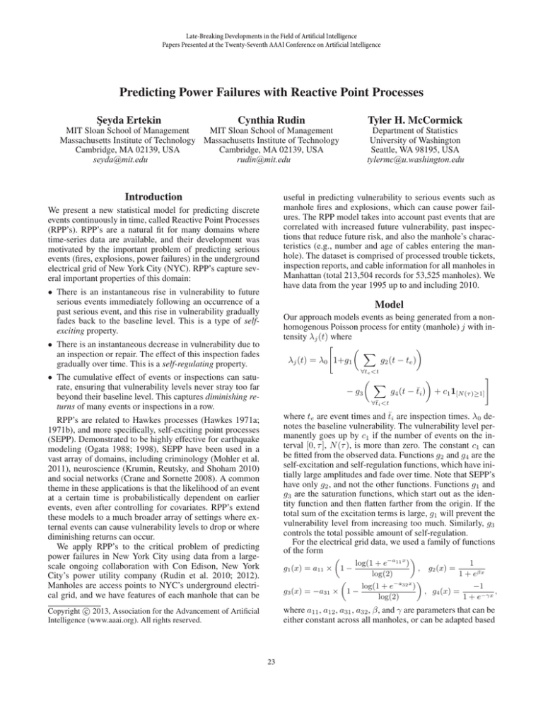
Late-Breaking Developments in the Field of Artificial Intelligence
Papers Presented at the Twenty-Seventh AAAI Conference on Artificial Intelligence
Predicting Power Failures with Reactive Point Processes
Şeyda Ertekin
Tyler H. McCormick
Cynthia Rudin
Department of Statistics
University of Washington
Seattle, WA 98195, USA
tylermc@u.washington.edu
MIT Sloan School of Management
MIT Sloan School of Management
Massachusetts Institute of Technology Massachusetts Institute of Technology
Cambridge, MA 02139, USA
Cambridge, MA 02139, USA
rudin@mit.edu
seyda@mit.edu
Introduction
useful in predicting vulnerability to serious events such as
manhole fires and explosions, which can cause power failures. The RPP model takes into account past events that are
correlated with increased future vulnerability, past inspections that reduce future risk, and also the manhole’s characteristics (e.g., number and age of cables entering the manhole). The dataset is comprised of processed trouble tickets,
inspection reports, and cable information for all manholes in
Manhattan (total 213,504 records for 53,525 manholes). We
have data from the year 1995 up to and including 2010.
We present a new statistical model for predicting discrete
events continuously in time, called Reactive Point Processes
(RPP’s). RPP’s are a natural fit for many domains where
time-series data are available, and their development was
motivated by the important problem of predicting serious
events (fires, explosions, power failures) in the underground
electrical grid of New York City (NYC). RPP’s capture several important properties of this domain:
• There is an instantaneous rise in vulnerability to future
serious events immediately following an occurrence of a
past serious event, and this rise in vulnerability gradually
fades back to the baseline level. This is a type of selfexciting property.
Model
Our approach models events as being generated from a nonhomogenous Poisson process for entity (manhole) j with intensity λj (t) where
"
X
λj (t) = λ0 1+g1
g2 (t − te )
• There is an instantaneous decrease in vulnerability due to
an inspection or repair. The effect of this inspection fades
gradually over time. This is a self-regulating property.
∀te <t
• The cumulative effect of events or inspections can saturate, ensuring that vulnerability levels never stray too far
beyond their baseline level. This captures diminishing returns of many events or inspections in a row.
− g3
X
#
g4 (t − t̄i ) + c1 1[N (τ )≥1]
∀t̄i <t
where te are event times and t̄i are inspection times. λ0 denotes the baseline vulnerability. The vulnerability level permanently goes up by c1 if the number of events on the interval [0, τ ], N (τ ), is more than zero. The constant c1 can
be fitted from the observed data. Functions g2 and g4 are the
self-excitation and self-regulation functions, which have initially large amplitudes and fade over time. Note that SEPP’s
have only g2 , and not the other functions. Functions g1 and
g3 are the saturation functions, which start out as the identity function and then flatten farther from the origin. If the
total sum of the excitation terms is large, g1 will prevent the
vulnerability level from increasing too much. Similarly, g3
controls the total possible amount of self-regulation.
For the electrical grid data, we used a family of functions
of the form
RPP’s are related to Hawkes processes (Hawkes 1971a;
1971b), and more specifically, self-exciting point processes
(SEPP). Demonstrated to be highly effective for earthquake
modeling (Ogata 1988; 1998), SEPP have been used in a
vast array of domains, including criminology (Mohler et al.
2011), neuroscience (Krumin, Reutsky, and Shoham 2010)
and social networks (Crane and Sornette 2008). A common
theme in these applications is that the likelihood of an event
at a certain time is probabilistically dependent on earlier
events, even after controlling for covariates. RPP’s extend
these models to a much broader array of settings where external events can cause vulnerability levels to drop or where
diminishing returns can occur.
We apply RPP’s to the critical problem of predicting
power failures in New York City using data from a largescale ongoing collaboration with Con Edison, New York
City’s power utility company (Rudin et al. 2010; 2012).
Manholes are access points to NYC’s underground electrical grid, and we have features of each manhole that can be
log(1 + e−a11 x )
1
g1 (x) = a11 × 1 −
, g2 (x) =
log(2)
1 + eβx
log(1 + e−a32 x )
−1
g3 (x) = −a31 × 1 −
, g4 (x) =
,
log(2)
1 + e−γx
where a11 , a12 , a31 , a32 , β, and γ are parameters that can be
either constant across all manholes, or can be adapted based
c 2013, Association for the Advancement of Artificial
Copyright Intelligence (www.aaai.org). All rights reserved.
23
g2 values from case control
fitted g2
15
g1 values from case control
fitted g1
20
10
4
2
5
0
0
−10
−10
0
−2
0
10
10
Age
6
Age
8
200
400
Number of Days
(a) Fitted g2
600
0
0.52
1.57
2.61
Bin Ranges
3.66
4.70
(b) Fitted g1
10
0
Main PH
−10
−20
0 −10
10 Total
Num Sets
(c) KL Divergence
10 0
−10
−10
10 0
Main PH −20 20 Total Num. Sets
(d) Log-Likelihood
Figure 1: Results for the Manhattan Dataset. Figures 1(a) and 1(b) show the fitted functions for the Manhattan dataset from
Case Control. Figures 1(c) and 1(d) show the KL Divergence from ABC and the Log-Likelihood, respectively.
on the manhole’s features. For instance, our experimental
analysis covers both constant β across all manholes as well
as an adaptive β, modeled for manhole k as:
Pn
βk = log 1 + e− i=1 θi fik
We use KL Divergence to measure differences in the distribution of time between events for the observed data and
the distribution of time between events generated using our
candidate parameter values. In Figure 1(c) the blue boundary corresponds to the region that yields the minimum divergence, and the optimum parameter values can be derived by
fitting a manifold on that region.
We also experimented with model fitting using Maximum
Likelihood techniques. Figure 1(d) demonstrates the region
of maximum likelihood (shown in dark red), where the simulated vulnerabilities are in closest proximity of actual vulnerabilities.
where θi is the coefficient of feature i and fik is the value of
feature i for manhole k. For our dataset, the features include
the number of main phase cables, age of the oldest cable,
and the total number of cable sets inside the manhole.
Model Fitting and Experiments
We will introduce several methods for fitting RPP’s below.
To verify that the methods are working properly, we used
simulated data where ground truth was available (not shown
here) to demonstrate that the underlying function could be
recovered.
Prediction Performance Evaluation
We assessed the predictive performance of our RPP model
by comparing it against Cox Proportional Hazards Model
(Cox 1972), which is a commonly used technique in survival analysis. We trained both an RPP model and a Cox
model (available in the survival package in R) on the historical event records up to the year 2010 and used the models
to predict vulnerabilities of each manhole on each day of
2010. We then generated a ranked list of manholes for each
day with the most vulnerable manhole ranked at the top. For
each manhole that had an event during a day, we compared
the rank of that manhole in the two ranked lists. Aggregated
over days in 2010 where an event was recorded, the RPP
model ranked the manholes with events significantly higher
than the Cox model in its lists, indicating that the RPP model
more accurately measures short term vulnerabilities.
Case Control
The Case Control method allows us to nonparametrically
trace out the shapes of g1 , g2 , g3 , and g4 , using only relevant manholes to estimate specific points of each function.
Figures 1(a) and 1(b) show g2 and g1 from Manhattan manholes, traced out (in blue) using the Case Control method,
and parameterized (in
P red) afterwards. For the g1 curve, the
range of observed
g2 values in the data was discretized
into equal sized bins, and the likelihood of an event if the
sum value falls within the range of a bin was used to fit g1 .
Bayesian and Maximum Likelihood Approaches
The Case Control method is useful for finding parameterizations of the functions, but there are not enough data to permit
its use when we would like to customize g1 , g2 , g3 , and g4 to
each individual manhole. Based on insights gleaned from the
Case Control method we explore both Bayesian and Maximum Likelihood approaches to model fitting.
For our Bayesian approach, we use the model for the βk ’s
with covariates described above, where each coefficient has
a Gaussian prior distribution. We fit the model using Approximate Bayesian Computation (ABC). To do this, we
evaluated the suitability of simulated data generated using
a given candidate parameter via two statistics, one consisting of the number of events and another related to the distribution of time between events. Since RPP’s model association between event times, the second statistic is important.
Understanding the Impact of Inspection Policies
Beyond identifying the vulnerable manholes to be targeted
for repair and inspection, we used the RPP model to simulate the effect of different broad inspection policies. Our
simulations show that there is a natural inverse relationship
between the number of events and the number of inspections: more inspections lead to fewer events. Using our simulations, we can quantify an optimal trade off between the
anticipated number of events and the cost of inspections.
This can assist Con Edison to make decisions between candidate inspection policies.
24
References
Cox, D. R. 1972. Regression models and life-tables. Journal
of the Royal Statistical Society. Series B (Methodological)
187–220.
Crane, R., and Sornette, D. 2008. Robust dynamic classes
revealed by measuring the response function of a social
system. Proceedings of the National Academy of Sciences
105(41):15649–15653.
Mohler, G.; Short, M.; Brantingham, P.; Schoenberg, F.;
and Tita, G. 2011. Self-exciting point process modeling
of crime. Journal of the American Statistical Association
106(493):100–108.
Krumin, M.; Reutsky, I.; and Shoham, S. 2010. Correlationbased analysis and generation of multiple spike trains using
Hawkes models with an exogenous input. Frontiers in computational neuroscience 4.
Ogata, Y. 1988. Statistical Models for Earthquake Occurrences and Residual Analysis for Point Processes. Journal
of the American Statistical Association 83(401):9–27.
Ogata, Y. 1998. Space-time point-process models for earthquake occurrences. Annals of the Institute of Statistical
Mathematics 50(2):379–402.
Rudin, C.; Passonneau, R.; Radeva, A.; Dutta, H.; Ierome,
S.; and Isaac, D. 2010. A process for predicting manhole
events in Manhattan. Machine Learning 80:1–31.
Rudin, C.; Waltz, D.; Anderson, R. N.; Boulanger, A.;
Salleb-Aouissi, A.; Chow, M.; Dutta, H.; Gross, P.; Huang,
B.; Ierome, S.; Isaac, D.; Kressner, A.; Passonneau, R. J.;
Radeva, A.; and Wu, L. 2012. Machine learning for the
New York City power grid. IEEE Transactions on Pattern
Analysis and Machine Intelligence 34(2):328–345.
Hawkes, A. 1971. Spectra of some self-exciting and mutually exciting point processes. Biometrika 58(1):83–90.
Hawkes, A. 1971. Point Spectra of Some Mutually Exciting Point Processes. Journal of the Royal Statistical Society
33(3):438–443.
25