Proceedings of the Thirtieth AAAI Conference on Artificial Intelligence (AAAI-16)
Decision Sum-Product-Max Networks
§
Mazen Melibari,§ Pascal Poupart,§ Prashant Doshi,‡
David R. Cheriton School of Computer Science, University of Waterloo, Canada
‡
Dept. of Computer Science, University of Georgia, Athens, GA 30602, USA
§
{mmelibar,ppoupart}@uwaterloo.ca, ‡ pdoshi@cs.uga.edu
Abstract
Sum-Product Networks (SPNs) were recently proposed as a
new class of probabilistic graphical models that guarantee
tractable inference, even on models with high-treewidth. In
this paper, we propose a new extension to SPNs, called Decision Sum-Product-Max Networks (Decision-SPMNs), that
makes SPNs suitable for discrete multi-stage decision problems. We present an algorithm that solves Decision-SPMNs
in a time that is linear in the size of the network. We also
present algorithms to learn the parameters of the network
from data.
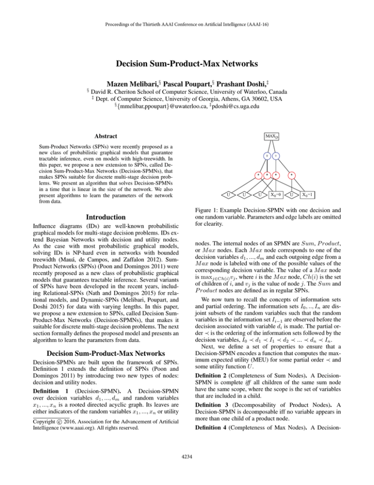
Figure 1: Example Decision-SPMN with one decision and
one random variable. Parameters and edge labels are omitted
for clearity.
Introduction
Influence diagrams (IDs) are well-known probabilistic
graphical models for multi-stage decision problems. IDs extend Bayesian Networks with decision and utility nodes.
As the case with most probabilistic graphical models,
solving IDs is NP-hard even in networks with bounded
treewidth (Mauá, de Campos, and Zaffalon 2012). SumProduct Networks (SPNs) (Poon and Domingos 2011) were
recently proposed as a new class of probabilistic graphical
models that guarantees tractable inference. Several variants
of SPNs have been developed in the recent years, including Relational-SPNs (Nath and Domingos 2015) for relational models, and Dynamic-SPNs (Melibari, Poupart, and
Doshi 2015) for data with varying lengths. In this paper,
we propose a new extension to SPNs, called Decision SumProduct-Max Networks (Decision-SPMNs), that makes it
suitable for discrete multi-stage decision problems. The next
section formally defines the proposed model and presents an
algorithm to learn the parameters from data.
nodes. The internal nodes of an SPMN are Sum, P roduct,
or M ax nodes. Each M ax node corresponds to one of the
decision variables d1 , ..., dm and each outgoing edge from a
M ax node is labeled with one of the possible values of the
corresponding decision variable. The value of a M ax node
is maxj∈Ch(i) vj , where i is the M ax node, Ch(i) is the set
of children of i, and vj is the value of node j. The Sum and
P roduct nodes are defined as in regular SPNs.
We now turn to recall the concepts of information sets
and partial ordering. The information sets I0 , .., In are disjoint subsets of the random variables such that the random
variables in the information set Ii−1 are observed before the
decision associated with variable di is made. The partial order ≺ is the ordering of the information sets followed by the
decision variables, I0 ≺ d1 ≺ I1 ≺ d2 ≺ ... ≺ dn ≺ In .
Next, we define a set of properties to ensure that a
Decision-SPMN encodes a function that computes the maximum expected utility (MEU) for some partial order ≺ and
some utility function U .
Decision Sum-Product-Max Networks
Decision-SPMNs are built upon the framework of SPNs.
Definition 1 extends the definition of SPNs (Poon and
Domingos 2011) by introducing two new types of nodes:
decision and utility nodes.
Definition 1 (Decision-SPMN). A Decision-SPMN
over decision variables d1 , ..., dm and random variables
x1 , ..., xn is a rooted directed acyclic graph. Its leaves are
either indicators of the random variables x1 , ..., xn or utility
Definition 2 (Completeness of Sum Nodes). A DecisionSPMN is complete iff all children of the same sum node
have the same scope, where the scope is the set of variables
that are included in a child.
Definition 3 (Decomposability of Product Nodes). A
Decision-SPMN is decomposable iff no variable appears in
more than one child of a product node.
c 2016, Association for the Advancement of Artificial
Copyright Intelligence (www.aaai.org). All rights reserved.
Definition 4 (Completeness of Max Nodes). A Decision-
4234
SPMN is max-complete iff all children of the same max
node have the same scope, where the scope is the set of decision variables that are included in a child.
Definition 5 (Uniqueness of Max Nodes). A DecisionSPMN is max-unique iff each max node that corresponds
to a decision variable d appears at most once in every path
from root to leaves.
We can obtain the maximum expected utility of a decision problem that has the partial order ≺ and utility function U using the Sum-Max-Sum rule, in which we alternate
between summing over the variables in an information set
and maximizing over a decision variable. The next definition makes a connection between Decision-SPMNs and the
Sum-Max-Sum rule. We use the notion S(e) to indicate the
value of a Decision-SPMN when evaluated at evidence e.
Definition 6. A Decision-SPMN S is valid iff S(e) =
MEU(e| ≺, U)
Figure 1 shows an example of a Decision-SPMN over
a decision variable, D, and a random variable, X0 . Solving a Decision-SPMN can be done by setting the indicators
that are compatible with the evidence to 1 and the rest to 0,
then performing a bottom-up pass on the network. The optimal strategy can be found by tracing back the network and
choosing the edges that maximize the decision nodes.
specific-scope of each node to its parents can be used to define the specific-scope of all the nodes in a SPMN.
For each unique instance Di in D we perform a top-down
pass, where we follow all the nodes that have values consistent with Di in their specific-scope. If we reach a utility
node, then we set its value to the utility value in Di .
Learning the Embedded Probability Distribution The
second sub-task is to learn the parameters of the embedded
probability distribution. In particular, we seek to learn the
weights of the sum nodes. This can be done using a special derivation of the Expectation-Maximization (EM) algorithm that is suitable for SPMNs. For each instance, Di , in
the dataset, we set the indicators to their values in Xi (the
observed values of the random variables in instance Di ).
We then perform inference by evaluating the SPMN using
a bottom-up pass. In order to integrate the decisions, D, for
instance Di , each max node will multiply the value of its
children with either 0 or 1 depending on the value of the
corresponding decision in the instance. This multiplication
is equivalent to augmenting the SPMN with indicators for
the max nodes. And since we are only concerned with the
weights of the sum nodes in this sub-task, all the utility
nodes can be treated as hidden variables with fixed probability distributions, where summing them out will always
result in the value 1. We also perform a top-down pass to
compute the gradient of the nodes. The expected counts of
each child of a sum node is maintained using a counter for
each child. We normalize and assign those values to the sum
nodes at the end of each iteration. This process is repeated
until convergence.
Parameters Learning
Let D be a dataset that consists of |D| instances, where
each instance, Di , is a tuple of the values of observed
random variables, X, the values of decision variables, D,
and a single utility value, u, that represents the utility of
the joint assignment of values for X and D; i.e. Di =
X, D, U (X, D). Algorithm 1 gives an overview of the parameter learning process. The process is split into two subtasks: 1) Learning the values of the utility nodes, 2) Learning
the embedded probability distribution. The following sections describe these two sub-tasks in detail.
Conclusion and Future Work
We proposed a new extension to SPNs, called Decision Sum-Product-Max Networks (Decision-SPMNs), that
makes SPNs suitable for discrete multi-stage decision problems. Solving Decision-SPMNs can be done in a time that is
linear in the size of the network. We also presented an algorithm to learn the parameters of the network from data. An
important direction for future work is to develop an efficient
structure learning algorithm for Decision-SPMNs. Another
future work is to experimentally evaluate how DecisionSPMNs and alternative discrete multi-stage decision models
can perform on real-life datasets.
Algorithm 1: Decision-SPMN Parameters Learning
input : S: Decision-SPMN, D: Dataset
output: Decision-SPMN with learned parameters
S ← learnUtilityValues(S, D);
S ← decisionSpmnEM(S, D);
References
Mauá, D. D.; de Campos, C. P.; and Zaffalon, M. 2012. The
complexity of approximately solving influence diagrams. In
Twenty-Eighth Conference on Uncertainty in Artificial Intelligence (UAI-12), 604–613. AUAI Press.
Melibari, M.; Poupart, P.; and Doshi, P. 2015. Dynamic Sum
Product Networks for Tractable Inference on Sequence Data.
ArXiv e-prints.
Nath, A., and Domingos, P. 2015. Learning relational sumproduct networks. In Twenty-Ninth AAAI Conference on Artificial Intelligence.
Poon, H., and Domingos, P. 2011. Sum-product networks: A
new deep architecture. In Proc. 12th Conf. on Uncertainty in
Artificial Intelligence, 2551–2558.
Learning the Values of the Utility Nodes The first subtask is to learn the values of the utility nodes. We start by
introducing the notion of specific-scope. The specific-scope
for an indicator node is the value of the random variable
that the indicator represents; for all other nodes the specificscope is the union of their childrens’ specific-scopes. For example, an indicator node, Ix , for X = x has the specificscope {x}, while an indicator node, Ix̄ , for X = x̄ has
the specific-scope {x̄}. A sum node over Ix and Ix̄ has the
specific-scope {x, x̄}. A product node that has two children,
one with specific-scope {x, x̄} and another one with specificscope {y}, will have the specific-scope {x, x̄, y}. A simple
algorithm that performs a bottom-up pass and propagates the
4235