Proceedings of the Thirtieth AAAI Conference on Artificial Intelligence (AAAI-16)
SAND: Semi-Supervised Adaptive Novel
Class Detection and Classification over Data Stream
Ahsanul Haque and Latifur Khan
Michael Baron
Department of Computer Science
The University of Texas at Dallas
Richardson, Texas 75080
Email: {ahsanul.haque, lkhan}@utdallas.edu
Department of Mathematical Sciences
The University of Texas at Dallas
Richardson, Texas 75080
Email: mbaron@utdallas.edu
by a user or a human annotator. Therefore, given the constraint of time and resource, it is not feasible to have true
labels for all instances in a data stream available. Concept
Evolution occurs when a new class emerges in any data
stream (Masud et al. 2011). It has received less attention
than concept drift problem in the literature. Therefore, most
approaches misclassify novel class instances as one of the
existing classes, and increase the classification error.
We propose a framework in this paper which addresses
all of the above challenges. A change detection technique
(CDT) is used in the framework to detect any concept drift
and chunk boundary immediately. However, unlike existing approaches, it employs two unsupervised estimators
(namely, Purity and Association) to calculate classifier confidence in predictions, and applies the CDT on confidence
scores. Therefore, the proposed CDT is fully unsupervised.
To further reduce the execution time, we have proposed two
strategies to execute CDT selectively without losing classification accuracy.
The proposed framework maintains an ensemble of
clustering-based classifier models, each trained on a different dynamically determined partially labeled chunk of data.
Motivated by the principle of Uncertainty Sampling (Settles 2009), our framework reuses classifier confidence scores
calculated during prediction to select a few data instances
for labeling. The classifier is then updated using this limited
amount of labeled data without adding any extra overhead.
Our framework incorporates a novel class detector for
handling concept evolution. The detector assumes appearance of a single novel class at a time. Any instance falling
outside of decision boundary of the ensemble classifier is
identified as an outlier. The framework interprets presence
of sufficiently large number of outliers with strong cohesion
among themselves as emergence of a novel class.
Primary contributions of our work are as follows: 1) We
present an unsupervised technique to estimate classifier confidence in predicting labels of data instances. We theoretically justify choice of the estimators. 2) We design a suitable change detection technique for this specific scenario. 3)
To update the classifier, we use a limited amount of labeled
data selected without any extra overhead by reusing classifier confidence scores calculated during prediction. 4) We
present a semi-supervised framework which uses dynamically determined chunks to address both of concept drift
Abstract
Most approaches to classifying data streams either divide
the stream into fixed-size chunks or use gradual forgetting.
Due to evolving nature of data streams, finding a proper size
or choosing a forgetting rate without prior knowledge about
time-scale of change is not a trivial task. These approaches
hence suffer from a trade-off between performance and sensitivity. Existing dynamic sliding window based approaches
address this problem by tracking changes in classifier error
rate, but are supervised in nature. We propose an efficient
semi-supervised framework in this paper which uses change
detection on classifier confidence to detect concept drifts, and
to determine chunk boundaries dynamically. It also addresses
concept evolution problem by detecting outliers having strong
cohesion among themselves. Experiment results on benchmark and synthetic data sets show effectiveness of the proposed approach.
1
Introduction
As technological advancement continues to pave the path
for Internet of Things (IoT), mining data streams is becoming increasingly important. However, data stream mining is challenging due to large volume and high velocity of
data. Furthermore, certain properties of data streams distinguish themselves from traditional data mining, namely infinite length, concept drift, concept evolution, limited amount
of labeled data etc. (Haque, Khan, and Baron 2015b).
Infinite length problem of data streams is typically addressed by dividing the stream into fixed-size chunks,
e.g., (Parker and Khan 2015) or using gradual forgetting,
e.g., (Klinkenberg 2004). Since data streams are evolving in
nature, without prior knowledge of the time-scale of change,
both strategies suffer from a trade-off between performance
and sensitivity. Concept drift occurs when the target class
or concept evolves within the feature space in such a way
that the class encroaches or crosses previously defined decision boundaries. This challenge is addressed by updating the
classifier periodically, e.g., (Masud et al. 2011) or by using
an explicit change detector, e.g., (Bifet and Gavald 2007) to
decide when an update is necessary. These approaches assume that true labels for all data instances are readily available. However, typically true labels are provided manually
c 2016, Association for the Advancement of Artificial
Copyright Intelligence (www.aaai.org). All rights reserved.
1652
and concept evolution effectively. We employ several strategies for selective execution of CDT to reduce the execution
time of the proposed framework. 5) We evaluate our proposed framework on several benchmark and synthetic data
sets. Experiment results show that our framework exhibits
competitive performance compared with other state-of-theart approaches, regardless of using limited amount of labeled
data instances.
The rest of the paper is organized as follows: In Section 2,
we briefly discuss some related work. Section 3 describes
our approach in detail. We describe the data sets, evaluation
metrics and present experiment results in Section 4. Finally,
Section 5 concludes the paper.
2
data instances be readily available. This assumption is not
practical in the context of data streams (Masud et al. 2008).
Our proposed CDT detects change in classifier confidence,
which does not require any supervised information.
Existing semi-supervised approaches to classifying data
streams use active learning, computational geometry etc.
to select important data instances for labeling. For example, complex active learning is used in (Masud et al. 2010;
Zhu et al. 2007; Fan et al. 2004). Computational geometry
based approach COMPOSE (Dyer, Capo, and Polikar 2014)
can only address gradual (limited) drift, rather than abrupt
drift. Our proposed approach reuses the same confidence
scores calculated during prediction to select instances for labeling without adding any extra overhead.
Cluster based single class novelty detection methods
have been proposed in (Spinosa, de Leon, and Gama 2009;
Hayat and Hashemi 2010), which are not suitable for multiclass environment. (Masud et al. 2011) propose an approach
for multi-class novelty detection but use fixed-size chunks,
hence suffering from the trade-off discussed earlier. Unlike these approaches, our proposed approach uses dynamic
chunks for multi-class novelty detection.
Related Work
Approaches that divide data streams into fixed-size chunks,
e.g., (Parker and Khan 2015) cannot capture concept drift
immediately if the chunk size is too large, or suffer from unnecessary frequent training during stable time period if the
chunk size is too small (Bifet and Gavald 2007). Gradual
forgetting is also used in the literature, e.g., (Klinkenberg
2004) to address the infinite length problem of data streams.
However, finding the perfect decay function for mining an
evolving data stream is a challenge. In this paper, we use
an explicit change detection technique (CDT) to detect any
change of concept, and to determine the chunk size dynamically.
In data stream mining, CDT is used either to detect a
change in the input data distribution, or to detect a change
in the classifier feedback. Several methods, e.g., (Song et al.
2007; Kuncheva and Faithfull 2013) exist to detect change
of the input data distribution in a data stream. However, detecting change in a multidimensional space is a hard problem (Harel et al. 2014). It introduces error while finding
changes in the multidimensional input space, hence not efficient in the context of data stream mining. In this paper,
we focus on detecting change in one dimensional classifier
confidence.
Various CDTs have been proposed in the literature to detect concept drift from any significant change in the classifier
feedback. Adwin (Bifet and Gavald 2007) is a sliding window based technique that determines the size of the window
according to the rate of change observed from the window
data itself. (Gama et al. 2004) detects a change when the error rate over the whole current window significantly exceeds
the lowest error rate recorded. (Cieslak and Chawla 2007)
exploits Kruskal Wallis analysis and Kolmogorov Smirnov
tests to detect changes. (Harel et al. 2014) is based on obtaining statistics from the loss distribution of the learning algorithm by reusing the data multiple times via re-sampling.
Concept drift detection in (Alippi, Boracchi, and Roveri
2013) contains two CDTs based on ICI (Intersection of confidence intervals), one to detect change in the input data distribution and another to detect change in the classifier error
rate. Considering the large volume and high speed of today’s
data streams, running two CDTs after testing each instance
is expensive. Another ICI based approach is ACE (Nishida,
Yamauchi, and Omori 2005). All of the above CDTs detect
change in the classifier error rate, requiring true labels of all
Figure 1: High level work flow of SAND
3
Proposed Approach
Our proposed framework uses a semi-supervised ensemble
classifier consisting of k-NN type models for classification.
Instead of applying change detection technique (CDT) on
the classifier error rate, we apply CDT on classifier confidence estimates to detect concept drift, and the chunk
boundary. Subsequently, our approach requests labels for a
limited amount of instances based on the classifier confidence estimates to update the classifier. We also integrate
a novel class detector in our framework. This framework
will henceforth be referred to as “SAND” (Semi-Supervised
Adaptive Novel Class Detection and Classification over
Data Stream).
1653
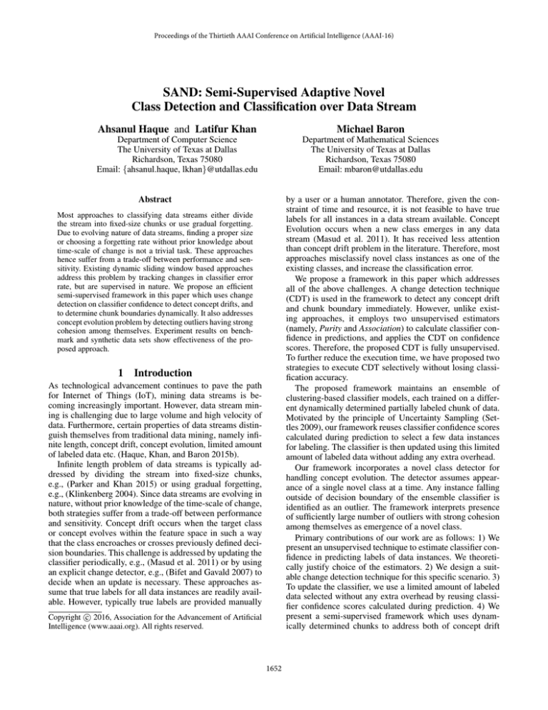
High level workflow of SAND is depicted in Figure 1.
The framework has four modules, i.e., Classification, Novel
Class Detection, Change Detection, and Update. SAND
maintains an ensemble M of t classification models, and
a dynamic window W containing classifier confidence estimates in predicting labels of test data instances. Let
{M1 , ..., Mt } be the models in the ensemble. At the beginning, the ensemble classifier contains models trained on the
initial training data. Once the warm up period is over, each
incoming instance in the data stream is first examined to
determine whether it is an outlier or not. It detects an instance as an outlier if the instance falls outside of the decision boundary of the ensemble classifier. If the instance is
not an outlier, it is classified as instance of an existing class
using majority voting among the models in the ensemble.
On the contrary, if the instance is an outlier, it is temporarily stored in a buffer. When there are enough instances in
the buffer, the Novel Class Detection module is invoked. We
define a class as novel class if none of the models in the ensemble has been trained with any instance from that class. If
a novel class is detected, the instances of the novel class are
tagged accordingly. Otherwise, the instances in the buffer
are considered as from existing classes and classified using
the current ensemble classifier. Details on training, classifier
decision boundary, classification and novel class detection
processes will be discussed later in this Section.
As soon as any test instance arrives, SAND along with
predicting the label of the instance, also estimates the confidence in the prediction. These confidence scores are stored
in W . Following insertion of a confidence estimate, the
Change Detection module searches for any change of distribution in the values stored in W . If it detects any significant
change in the confidence estimates, i.e., values stored in W ,
SAND assumes that a concept drift has occurred, and determines a chunk boundary immediately. Next, the classifier
needs to be updated to adapt to the changed concept. To form
the training data, SAND requests true labels for instances
in the current data chunk on which the classifier showed
weak confidence during prediction. For rest of the instances,
it uses the predicted labels as the final labels and includes
them in the training data. Finally, a new model is trained
on the training data, the ensemble is updated by including
the newly trained model, and W is reinitialized. On the contrary, if the Change Detection module finds no significant
change in the confidence scores, the current ensemble is retained and W keeps growing. Based on memory resource
available, we set a maximum size Smax for W . If W grows
beyond Smax , ensemble classifier is updated and W is reinitialized. Later in this Section, we discuss about calculation
of confidence scores and Change Detection module. Due to
limited space in this paper, more details on SAND along
with a list of frequently used symbols have been provided
in the technical report (Haque, Khan, and Baron 2015a).
3.1
ing data is required to be labeled to build the models. In our
experiments, we use an impurity based K-means clustering
algorithm (details in (Haque, Khan, and Baron 2015a)). We
set the value of K based on the size of the training data. Raw
data points are discarded after saving summaries (mentioned
as pseudopoints) of the clusters. Therefore, each model Mi
is a collection of K pseudopoints. Summary of a cluster,
i.e., a pseudopoint contains centroid, radius, and number of
data points belonging to each of the classes (referred to as
frequencies). Radius of a cluster is defined as the distance
between the centroid and the farthest data point in that cluster. A test instance x is classified using Mi as follows. Let
h ∈ Mi be the pseudopoint whose centroid is the nearest
from x. The predicted class of x is the class that has the
highest frequency in h. The data point x is classified using
the ensemble M by taking majority vote among all classifiers.
Each pseudopoint corresponds to a “hypersphere” in the
feature space. The decision boundary of a model Mi is the
union of the feature spaces encompassed by all pseudopoints
h ∈ Mi . The decision boundary of the ensemble M is the
union of the decision boundaries of all models Mi ∈ M.
3.2
Novel Class Detection
Each test instance is first examined by the ensemble classifier M. If the instance is inside the decision boundary, it is
classified normally as described in Section 3.1. Otherwise,
it is declared as a filtered outlier, or F-outlier. The principle
behind the novel class detection is that a data point should be
closer to the data points of its own class (cohesion) and farther apart from the data points of other classes (separation).
Therefore, if there is a novel class in the stream, instances
belonging to that class will be far from the existing class
instances, and will be close to other novel class instances.
Since F-outliers are outside of the decision boundary, they
are far from the existing class instances. So, the separation property for a novel class is satisfied by the F-outliers.
Therefore, F-outliers are potential novel class instances, and
they are temporarily stored in a buffer to observe whether
they also satisfy the cohesion property. The buffer is examined periodically to see whether there are enough F-outliers
that are close to each other. This is done by computing the
q-Neighborhood Silhouette Coefficient, or q-NSC (Masud et
al. 2011). This is defined based on q, c-neighborhood of an
F-outlier x (q, c(x) in short), which is the set of q instances
from class c that are nearest to x. Here q is a user defined
parameter.
For example, q, c1 (x) of an F-outlier x is the q-nearest
class c1 neighbors of x. Let D̄cout ,q (x) be the mean distance
of an F-outlier x to its q-nearest F-outlier neighbors. Also,
let D̄c,q (x) be the mean distance from x to its q, c(x), and
let D̄cmin ,q (x) be the minimum among all D̄c,q (x), c ∈{Set
of existing classes}. In other words, q, cmin is the nearest
existing class neighborhood of x. Then q-NSC of x is given
by:
Training and Classification
Each model in the ensemble is based on the idea of k-NN.
Rather than storing the raw training data, a number of clusters are built using a clustering algorithm, e.g., K-means,
DBSCAN (Ester et al. 1996) etc. Only a portion of the train-
q-N SC(x) =
1654
D̄cmin ,q (x) − D̄cout ,q (x)
max(D̄cmin ,q (x), D̄cout ,q (x))
(1)
The expression q-NSC is a unified measure of cohesion
and separation, and yields a value between -1 and +1. A
positive value indicates that x is closer to the F-outlier instances (more cohesion) and farther away from existing class
instances (more separation), and vice versa. The q-NSC(x)
value of an F-outlier x must be computed separately for each
classifier Mi ∈ M. A new class is declared if there are at
least q (> q) F-outliers having positive q-NSC for all classifiers Mi ∈ M.
cm in hip .
Association and purity of the model Mi is denoted by Ai
and Pi respectively. Theoretical justification of these heuristics is provided in (Haque, Khan, and Baron 2015a). Both
of the heuristics contribute to model confidence according
to their estimation capability. This capability is measured
by the correlation between heuristic values and classification accuracy using the initial training instances as follows.
Heuristic values for Mi are calculated for each of the labeled
k
training instances. Let Hij
be the value of j th heuristic in
Mi ’s classification of instance k. Since we use two heuristics, j ∈ {1, 2}. Let ŷik be the prediction of Mi on instance k
and y k be the true label of that instance. Let vi be the vector
containing vik values indicating whether the classification of
instance k by model Mi is correct or not. In other words,
vik = 1 if ŷik = y k and vik = 0 if ŷik = y k . Finally, a correlation vector ri is calculated for model Mi . It contains rij
values which are pearson’s correlation coefficients between
Hij and vi for different j. No labeled data is required for
confidence estimation after initial training.
To calculate model confidence in the testing phase, SAND
first calculates heuristic values Hix for a test instance x. Let
Cix be the confidence of model Mi in predicting test instance
x. Next, Cix is calculated by taking the dot product of Hix and
ri calculated during initial training, i.e., Cix = Hix .ri . Similarly, SAND calculates confidence scores for each of the
models in the ensemble. These scores are then normalized
between 0 and 1. Finally, SAND takes the average confidence of the models towards the predicted class to estimate
confidence of the entire ensemble C x .
Algorithm 1 Change detection algorithm
1: W ← ∅ // Initialize W
2: Th ← −log(α) // α is sensitivity parameter
3: while true do
4:
[ŷ, C x ] ← Classify(x)
5:
W ⇐ C x // Enqueue C x into W
6:
N ← |W |; wn ← 0;
7:
ecp ← −1 // ecp contains the estimated change point
8:
for k ← Δ to N − Δ do
9:
mb ← mean(W [1 : k])
10:
ma ← mean(W [k + 1 : N ])
11:
if ma ≤ (1 − α) ∗ mb then
12:
Sk ← 0
13:
Beta[α̂b , β̂b ] ← estimateParam(W [1 : k])
14:
Beta[α̂a , β̂a ] ← estimateParam(W [k + 1 : N ])
15:
16:
17:
18:
19:
20:
21:
22:
23:
24:
25:
26:
27:
3.3
for i ← k + 1 to Ndo
f (W [i] | α̂a ,β̂a )
Sk ← Sk + log f W [i] | α̂ ,β̂
(
b b)
end for
if Sk > wn then
wn ← Sk
end if
end if
end for
if wn > Th then
UpdateClassifier(M, W, τ )
W ← ∅ // Reinitialize W
end if
end while
3.4
Change Detection
As discussed earlier, SAND maintains a variable size window W to monitor estimates of classifier confidence on recent data instances. These estimates tend to follow a beta
distribution which is confirmed by Chi-Square goodnessof-fit test. It can be shown theoretically that the classifier
confidence reduces consistently when there is a concept
drift (Haque, Khan, and Baron 2015a). A CDT is therefore
applied on W values to detect any significant change, i.e., a
concept drift.
We propose a CUSUM (Baron 1999)-type change detection technique (CDT) on beta distribution to use in this context. Algorithm 1 sketches the proposed CDT. As soon as
a new test instance arrives, along with predicting the label,
confidence of the classifier is estimated and stored in W
(Line 4 and Line 5). Next, the proposed CDT divides W into
two sub-windows for each k between Δ to N − Δ, where
N is the total number of observations in W . Let Wb and Wa
be the sub-windows respectively, where Wa contains confidence estimates on more recent instances. Each sub-window
is required to contain at least Δ number of values to preserve statistical properties of a distribution. When a concept
drift occurs, confidence scores are expected to decrease. So,
only changes in the negative direction are required to be detected. In other words, if ma and mb are the mean values of
the observations in Wa and Wb respectively, change point is
searched only if ma ≤ (1 − α) ∗ mb , where α is the sensi-
Calculation of Confidence Scores
First, two heuristics, i.e., association and purity are used to
estimate the confidence of each individual model. Next, individual model confidences are combined to estimate the overall confidence of the ensemble classifier which is stored in
W . Let hip be the pth pseudopoint in Mi , and cm be the class
having the highest frequency in hip . Assuming the closest
pseudopoint from an instance x in model Mi is hip , We define the heuristics as follows:
• Association is calculated by R(hip ) − Dip (x), where
R(hip ) is the radius of hip and Dip (x) is the distance of
x from hip . Therefore, smaller the Dip (x), higher the association.
|L (cm )|
• Purity is calculated by ip
|Lip | , where |Lip | is sum of all
the frequencies in hip and |Lip (cm )| is the frequency of
1655
tivity. We use α = 0.05 and Δ = 100 in our experiments,
which are also widely used in the literature.
It is known that the values in each sub-window tend to
follow a beta distribution. However, the actual parameter
values are unknown. The proposed CDT estimates these parameters at Line 13 and 14. Then, the sum of the log likelihood ratios Sk is calculated in the inner for loop between
Lines 15 and 17, where f (Xi , α̂, β̂) is the probability density function
(PDF) of the beta distribution having parameters α̂, β̂ applied on the data instance Xi . Next, a score
wn for all the values stored in W is calculated in the outer
for loop between Lines 8 and 22. Let kmax is the value of
k for which the algorithm calculated the maximum Sk value
where Δ ≤ k ≤ N − Δ. Finally, a change is detected at
point kmax if wn is greater than a pre-fixed threshold. We
use −log(α) as the threshold value. W is reinitialized and a
chunk boundary is determined if a change is detected, otherwise W keeps growing.
3.5
4
4.1
Data Sets
Table 1 depicts the characteristics of the data sets. ForestCover is obtained from the UCI repository as explained
in (Masud et al. 2011). We normalize the data set, and arrange the data in order to prepare it for novel class detection
so that in any chunk at most three and at least two classes
co-occur, and new classes appear randomly. For the second data set, we use Physical Activity Monitoring data set
(PAMAP) from UCI (Reiss and Stricker 2012). Powersupply (Zhu 2010) data set contains hourly power supply information of an Italian electricity company. HyperPlane (Zhu
2010) is a synthetic data stream which is generated using the
d−1 (x +x )
equation: f (x) = j=1 aj j xjj+1 , where f (x) is the label of instance x and aj , j = 1, 2, .., d, controls the shape
of the decision surfaces. SynRBF@X are synthetic data sets
generated using RandomRBFGeneratorDrift of MOA (Bifet
et al. 2010) framework, where X is the Speed of change
of centroids in the model. Therefore, increasing X refers to
more frequent concept drifts in the data set. We use ForestCover and PAMAP for simulating both concept drift and
novel classes. Rest of the data sets are used to test only concept drift handling capability of different approaches.
Updating the Ensemble using Limited
Labeled Data
Once a change is detected, the classifier is updated using
the recent chunk. However, instead of requiring true labels
of all the data instances, SAND intelligently selects a few
instances using the classifier confidence scores. First, if the
confidence is below the confidence threshold (τ ), SAND requests for its true label and includes it in the labeled instance
set. Otherwise, SAND uses the predicted label and includes
the instance in the unlabeled instance set. Next, the labeled
and unlabeled set of instances are used to form the training
data set. It is apparent that the value of τ is inversely proportional to the percentage of labeled data. Therefore, the value
of τ is set based on the availability of labeled instances. Finally, a new model is trained on the training data set. Detail
algorithm is provided in (Haque, Khan, and Baron 2015a).
Once a new model is trained, it replaces the oldest one
among the existing models in the ensemble. This ensures
that we have exactly t models in the ensemble at any time.
In this way, the infinite length problem is addressed because
a constant amount of memory is required to store the ensemble. The concept drift problem is addressed by keeping the
ensemble up-to-date with the most recent concept.
3.6
Experiment Results
Table 1: Characteristics of data sets
Name of
Num of
Num of Num of
Data set
Instances Classes Features
ForestCover
150,000
7
54
PAMAP
150,000
19
52
Power Supply
29,927
2
24
HyperPlane
100,000
5
10
SynRBF@0.002 100,000
7
70
SynRBF@0.003 100,000
7
70
4.2
Experiment Setup
We compare classification and novel class detection performance of SAND with ECSMiner (Masud et al. 2011).
We have chosen ECSMiner since it is a robust and efficient framework for classifying data streams, and addresses both of concept drift and concept evolution problems. Apart from that, we compare SAND with OzaBagAdwin (OBA) and Adaptive Hoeffding Tree (AHT) implemented in MOA (Bifet et al. 2010) framework. Both of OBA
and AHT use adwin (Bifet and Gavald 2007) as the change
detector. These approaches do not have novel class detection
feature. So, we compare these approaches with our approach
only in terms of classification performance.
We evaluate each of the above classifiers on a stream by
testing and then training with chunks of data in sequence. To
evaluate ECSMiner, we use 50 pseudopoints, ensemble size
6 as suggested in (Masud et al. 2011). We use 100% labeled
training data to evaluate ECSMiner, OBA and AHT. On the
other hand, we set t = 6 and q = 50 in SAND using cross
validation.
Run Time Reduction
Time complexity of SAND is analyzed in (Haque, Khan, and
Baron 2015a). The bottleneck of SAND is to invoke CDT
after inserting each confidence value in W . We examine the
following strategies for selective execution of the CDT:
1. CDT is executed if classifier confidence is below τ . This
will be referred to as SAND-F.
x
2. CDT is executed with a probability of e−C , i.e., higher
the confidence, lower the probability of executing CDT
and vice versa. This will be referred to as SAND-D.
1656
Name of
Data set
ForestCover
PAMAP
Power Supply
HyperPlane
SynRBF@0.002
SynRBF@0.003
Table 2: Summary of classification results
SAND-D (τ = 0.9) SAND-F (τ = 0.9) ECSMiner
Error%
Error%
Error%
3.75
6.445
4.55
4.26
4.817
35.26
0.02
0.02
0.05
0.01
0.02
3.73
32.13
20.035
63.43
34.61
25.886
65.39
AHT
Error%
22.89
8.76
85.59
46.24
38.75
48.65
OBA
Error%
18.06
7.27
86.92
48.55
37.04
46.86
Table 3: Comparison of classification performance using limited amount of labeled data
Name of
SAND-D (τ = 0.4)
SAND-F (τ = 0.4)
ECSMiner
AHT
Data Set
Error% % of labeled data Error% % of labeled data
Error%
Error%
ForestCover
4.69
45.26
4.91
32.86
4.55
22.89
PAMAP
5.11
70.72
5.13
69.80
35.26
8.76
Power Supply
0.03
0.122
0.05
0.1
0.05
85.59
HyperPlane
0.02
0.227
0.04
0.23
3.73
46.24
SynRBF@0.002
54.4
33.18
56.67
34.70
63.43
38.75
SynRBF@0.003
53.86
42.20
55.38
38.76
65.39
48.65
4.3
Performance Metrics
τ results in fewer labeled data instances. Results from Table 3 show that SAND-D and SAND-F using τ = 0.4
also show very competitive classification performance compared with other approaches, if not better, despite using very
limited amount of labeled data instances. Furthermore, we
observed from our experiment results (Haque, Khan, and
Baron 2015a) that SAND achieves speed up by using run
time reduction strategies stated in Section 3.6.
Let F N = total novel class instances misclassified as existing class, F P = total existing class instances misclassified as novel class, T P = total novel class instances correctly classified as novel class, F e = total existing class
instances misclassified (other than F P ), Nc = total novel
class instances in the stream, and N = total instances in
the stream. We use the following performance metrics to
evaluate our technique: 1) Error%: Total misclassification
error (percent), i.e., (F P +F NN+F e)∗100 . 2) Mnew : % of novel
.
class instances misclassified as existing class, i.e., F NN∗100
c
3) Fnew : % of existing class instances falsely identified as
∗100
novel class, i.e., FNP−N
.
c
4.4
OBA
Error%
18.06
7.27
86.92
48.55
37.04
46.86
Table 4: Summary of novel class detection results
Data set
ForestCover
PAMAP
Classification Performance
Unlike ECSMiner, SAND determines the chunk size dynamically based on changes in classifier confidence. Therefore, SAND avoids unnecessary training during stable period and frequently updates the classifier when needed. As
an instance, with increasing speed of change of centroids X
in SynRBF@X data sets, our proposed CPD helps SAND
to update the ensemble classifier more frequently to cope
up with more frequent concept drift. SAND-D (τ = 0.9)
creates 540 and 554 number of chunks while classifying
SynRBF@0.002 and SynRBF@0.003 respectively, where
ECSMiner creates same 47 number of chunks in both of
the cases. Further experiment results presented in (Haque,
Khan, and Baron 2015a) show that despite using limited labeled data, SAND successfully detects concept drifts and
updates the classifier timely.
Table 2 compares classification error of SAND-D (τ =
0.9) and SAND-F (τ = 0.9) with other baseline approaches.
SAND-D and SAND-F outperform other approaches in all
the cases. As mentioned in Section 3, increasing value of
4.5
Method
SAND-D (τ = 0.9)
SAND-F (τ =0.9)
ECSMiner
SAND-D (τ = 0.9)
SAND-F (τ =0.9)
ECSMiner
Mnew
8.525
12.427
8.417
0.048
0.049
0.047
Fnew
1.865
2.120
2.128
3.884
4.325
37.530
Novel Class Detection Performance
As discussed in Section 3.2, SAND detects emergence of a
novel class if it finds enough filtered outliers that are close to
each other. Similar to ECSMiner, we consider arrival of 400
instances as the maximum allowable time, until which the
classifier can wait to detect a emerging class (Masud et al.
2011). Table 4 compares novel class detection performance
of SAND-D and SAND-F using τ = 0.9 with ECSMiner
on different data sets. We observe that, SAND-D shows the
best Fnew and very competitive Mnew despite using a limited amount of labeled data. SAND-F can be used where
satisfactory result is required within tight time constraint by
adjusting the value of τ .
Experiment results presented in (Haque, Khan, and Baron
2015a) indicate that SAND is not excessively sensitive to the
parameters t and Smax . Considering overall performance
1657
(Error%, Mnew , and Fnew ), SAND clearly outperforms all
the other baseline approaches. Moreover, SAND can also
be very useful to save time and resources by using limited
amount of labeled data and by executing change detection
selectively, without sacrificing accuracy.
5
Haque, A.; Khan, L.; and Baron, M. 2015b. Semi supervised
adaptive framework for classifying evolving data stream. In
Advances in Knowledge Discovery and Data Mining, volume 9078 of Lecture Notes in Computer Science. Springer
International Publishing. 383–394.
Harel, M.; Mannor, S.; El-yaniv, R.; and Crammer, K. 2014.
Concept drift detection through resampling. In ICML-14,
1009–1017. JMLR Workshop and Conference Proceedings.
Hayat, M. Z., and Hashemi, M. R. 2010. A dct based
approach for detecting novelty and concept drift in data
streams. In SoCPaR, 373–378. IEEE.
Klinkenberg, R. 2004. Learning drifting concepts: Example selection vs. example weighting. Intell. Data Anal.
8(3):281–300.
Kuncheva, L. I., and Faithfull, W. J. 2013. PCA feature extraction for change detection in multidimensional unlabelled
data. IEEE Transactions on Neural Networks and Learning
Systems.
Masud, M. M.; Gao, J.; Khan, L.; Han, J.; and Thuraisingham, B. M. 2008. A practical approach to classify evolving
data streams: Training with limited amount of labeled data.
In ICDM, 929–934.
Masud, M.; Gao, J.; Khan, L.; Han, J.; and Thuraisingham,
B. 2010. Classification and novel class detection in data
streams with active mining. In Advances in Knowledge Discovery and Data Mining, volume 6119 of Lecture Notes in
Computer Science. Springer Berlin Heidelberg. 311–324.
Masud, M. M.; Gao, J.; Khan, L.; Han, J.; and Thuraisingham, B. M. 2011. Classification and novel class detection in
concept-drifting data streams under time constraints. IEEE
Trans. Knowl. Data Eng. 23(6):859–874.
Nishida, K.; Yamauchi, K.; and Omori, T. 2005. Ace: Adaptive classifiers-ensemble system for concept-drifting environments. In Multiple Classifier Systems, volume 3541 of
Lecture Notes in Computer Science, 176–185. Springer.
Parker, B., and Khan, L. 2015. Detecting and tracking concept class drift and emergence in non-stationary fast data
streams. In Twenty-Ninth AAAI Conference on Artificial Intelligence.
Reiss, A., and Stricker, D. 2012. Introducing a new benchmarked dataset for activity monitoring. In ISWC, 108–109.
IEEE.
Settles, B. 2009. Active learning literature survey. Computer
Sciences Technical Report 1648, University of Wisconsin–
Madison.
Song, X.; Wu, M.; Jermaine, C.; and Ranka, S. 2007. Statistical change detection for multi-dimensional data. In 13th
ACM SIGKDD, 667–676. NY, USA: ACM.
Spinosa, E. J.; de Leon, A. P.; and Gama, J. . 2009. Novelty
detection with application to data streams. Intell. Data Anal.
13:405–422.
Zhu, X.; Zhang, P.; Lin, X.; and Shi, Y. 2007. Active learning from data streams *. In International Conference on
Data Mining (ICDM), 757–762.
Zhu, X. 2010. Stream data mining repository. http://www.
cse.fau.edu/∼xqzhu/stream.html.
Conclusion
SAND is a semi-supervised framework which estimates
classifier confidence in predicting instances from any evolving data stream. It facilitates addressing of both concept
drift and concept evolution by detecting changes in classifier
confidence estimates, and dynamically determining chunk
boundaries. Several strategies have been proposed to further
reduce the execution time of SAND. Empirical results show
that, SAND is effective regardless of using only a limited
amount of labeled data.
Acknowledgments
This material is based upon work supported by NSF award
no. CNS-1229652 and DMS-1322353.
References
Alippi, C.; Boracchi, G.; and Roveri, M. 2013. Just-in-time
classifiers for recurrent concepts. IEEE Trans. Neural Netw.
Learning Syst. 24(4):620–634.
Baron, M. 1999. Convergence rates of change-point estimators and tail probabilities of the first-passage-time process.
Canadian J. of Statistics 27:183–197.
Bifet, A., and Gavald, R. 2007. Learning from timechanging data with adaptive windowing. In Proceedings of
SIAM International Conference on Data Mining. SIAM.
Bifet, A.; Holmes, G.; Pfahringer, B.; Kranen, P.; Kremer,
H.; Jansen, T.; and Seidl, T. 2010. Moa: Massive online
analysis, a framework for stream classification and clustering. In Journal of Machine Learning Research, 44–50.
Cieslak, D., and Chawla, N. 2007. Detecting fractures in
classifier performance. In ICDM 2007, 123–132.
Dyer, K. B.; Capo, R.; and Polikar, R. 2014. Compose:
A semisupervised learning framework for initially labeled
nonstationary streaming data. IEEE Transactions on Neural
Networks and Learning Systems 25(1):12 – 26.
Ester, M.; Kriegel, H.-P.; Sander, J.; and Xu, X. 1996.
A density-based algorithm for discovering clusters in large
spatial databases with noise. In Proc. of 2nd International
Conference on Knowledge Discovery and, 226–231.
Fan, W.; an Huang, Y.; Wang, H.; and Yu, P. S. 2004. Active
mining of data streams. In Proceedings of the Fourth SIAM
International Conference on Data Mining, 457–461.
Gama, J.; Medas, P.; Castillo, G.; and Rodrigues, P. 2004.
Learning with drift detection. In In SBIA Brazilian Symposium on Artificial Intelligence, 286–295. Springer Verlag.
Haque, A.; Khan, L.; and Baron, M. 2015a. Sand: Semi
supervised adaptive novel class detection and classification over data stream. Computer Science Technical Report
UTDCS-12-15, The University of Texas at Dallas.
1658