Proceedings of the Thirtieth AAAI Conference on Artificial Intelligence (AAAI-16)
Preferences Single-Peaked on Nice Trees
Dominik Peters and Edith Elkind
Department of Computer Science
University of Oxford, UK
{dominik.peters, edith.elkind}@cs.ox.ac.uk
j
Abstract
Preference profiles that are single-peaked on trees enjoy
desirable properties: they admit a Condorcet winner (Demange 1982), and there are hard voting problems that become
tractable on this domain (Yu, Chan, and Elkind 2013). Trick
(1989) proposed a polynomial-time algorithm that finds some
tree with respect to which a given preference profile is singlepeaked. However, some voting problems are only known to
be easy for profiles that are single-peaked on “nice” trees, and
Trick’s algorithm provides no guarantees on the properties of
the tree that it outputs. To overcome this issue, we build on the
work of Trick and Yu et al. to develop a structural approach
that enables us to compactly represent all trees with respect to
which a given profile is single-peaked. We show how to use
this representation to efficiently find the “best” tree for a given
profile, according to a number of criteria; for other criteria, we
obtain NP-hardness results. In particular, we show that it is
NP-hard to decide whether an input profile is single-peaked
with respect to a given tree. To demonstrate the applicability
of our framework, we use it to identify a new class of profiles
that admit an efficient algorithm for a popular variant of the
Chamberlin–Courant (1983) rule.
1
i
a
h
b
c
d
e
f
g
k
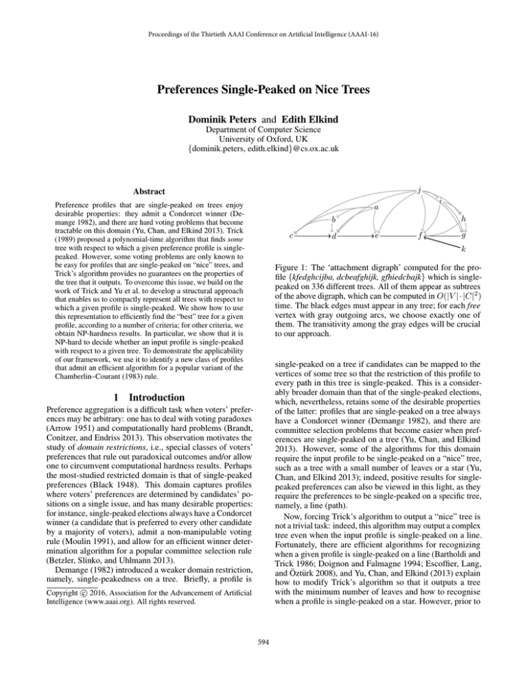
Figure 1: The ‘attachment digraph’ computed for the profile {kfedghcijba, dcbeafghijk, gfhiedcbajk} which is singlepeaked on 336 different trees. All of them appear as subtrees
of the above digraph, which can be computed in O(|V | · |C|2 )
time. The black edges must appear in any tree; for each free
vertex with gray outgoing arcs, we choose exactly one of
them. The transitivity among the gray edges will be crucial
to our approach.
single-peaked on a tree if candidates can be mapped to the
vertices of some tree so that the restriction of this profile to
every path in this tree is single-peaked. This is a considerably broader domain than that of the single-peaked elections,
which, nevertheless, retains some of the desirable properties
of the latter: profiles that are single-peaked on a tree always
have a Condorcet winner (Demange 1982), and there are
committee selection problems that become easier when preferences are single-peaked on a tree (Yu, Chan, and Elkind
2013). However, some of the algorithms for this domain
require the input profile to be single-peaked on a “nice” tree,
such as a tree with a small number of leaves or a star (Yu,
Chan, and Elkind 2013); indeed, positive results for singlepeaked preferences can also be viewed in this light, as they
require the preferences to be single-peaked on a specific tree,
namely, a line (path).
Now, forcing Trick’s algorithm to output a “nice” tree is
not a trivial task: indeed, this algorithm may output a complex
tree even when the input profile is single-peaked on a line.
Fortunately, there are efficient algorithms for recognizing
when a given profile is single-peaked on a line (Bartholdi and
Trick 1986; Doignon and Falmagne 1994; Escoffier, Lang,
and Öztürk 2008), and Yu, Chan, and Elkind (2013) explain
how to modify Trick’s algorithm so that it outputs a tree
with the minimum number of leaves and how to recognise
when a profile is single-peaked on a star. However, prior to
Introduction
Preference aggregation is a difficult task when voters’ preferences may be arbitrary: one has to deal with voting paradoxes
(Arrow 1951) and computationally hard problems (Brandt,
Conitzer, and Endriss 2013). This observation motivates the
study of domain restrictions, i.e., special classes of voters’
preferences that rule out paradoxical outcomes and/or allow
one to circumvent computational hardness results. Perhaps
the most-studied restricted domain is that of single-peaked
preferences (Black 1948). This domain captures profiles
where voters’ preferences are determined by candidates’ positions on a single issue, and has many desirable properties:
for instance, single-peaked elections always have a Condorcet
winner (a candidate that is preferred to every other candidate
by a majority of voters), admit a non-manipulable voting
rule (Moulin 1991), and allow for an efficient winner determination algorithm for a popular committee selection rule
(Betzler, Slinko, and Uhlmann 2013).
Demange (1982) introduced a weaker domain restriction,
namely, single-peakedness on a tree. Briefly, a profile is
c 2016, Association for the Advancement of Artificial
Copyright Intelligence (www.aaai.org). All rights reserved.
594
vertex has degree k. Note that paths are 2-regular (uniquely),
and the star K1,n is n-regular. A caterpillar is a tree in
which every vertex is within distance 1 of a central path; a
lobster is a tree in which every vertex is within distance 2
of a central path. A subdivision of a star is a tree obtained
from a star by replacing its edges by paths. The path-width
of a tree T is the minimum width of a tree decomposition of
T such that the underlying tree is a path (then called a path
decomposition); see, e.g., (Bodlaender 1994) for a definition
of a tree decomposition.
A profile V over C is single-peaked (on a line) if there is
a linear order on C such that for every v ∈ V , we have
x v y whenever v[1] x y or y x v[1] . V is
single-peaked on T , where T is a tree with vertex set C, if
V is single-peaked when restricted to the vertex set of every
path in T . Equivalently, V is single-peaked on T if for every
v ∈ V and each k = 1, . . . , |C|, the set v[1:k] induces a
subtree of T . Given a profile V , we denote the set of all
trees T such that V is single-peaked on T by T (V ); we say
that trees in T (V ) are suitable for V . A profile V over C
is single-peaked on a tree if T (V ) = ∅. In particular, V is
single-peaked on a line if and only if it is single-peaked on a
tree T that is a path.
A digraph D = (V, A) is a directed graph with no selfloops or multiple arcs. An arc (u, v) ∈ A points from its
tail u to its head v. We will write uv for (u, v). An acyclic
digraph (a dag) is a digraph with no directed cycles. For
a vertex v, its out-degree (resp., in-degree) d+ (v) (resp.,
d− (v)) is the number of arcs whose tail (resp., head) is v. A
sink is a vertex v with d+ (v) = 0, a source is a vertex with
d− (v) = 0. Every dag has at least one sink and one source.
Given a digraph D = (V, A), we can forget about its
orientation to obtain an underlying graph G = (V, E) where
{u, v} ∈ E if and only if uv ∈ A or vu ∈ A.
this work, no such algorithms were known for other types
of “nice” trees, such as trees that have bounded diameter or
a small number of internal nodes; in fact, it was an open
question whether, given a profile V and a tree T , one can
check in polynomial time whether V is single-peaked on T .
In this paper, we propose a general framework for answering such questions, and use it to obtain polynomial-time
algorithms for identifying “nice” trees when they exist, for
several appealing notions of “niceness”. Specifically, we
define a digraph that encodes, in a compact fashion, all trees
with respect to which a given profile is single-peaked, an
example is shown in Figure 1. This digraph enables us to
count and/or enumerate all such trees. Moreover, we show
that it has many useful structural properties, which can be
exploited to efficiently find trees that have, e.g., the minimum
degree, diameter, or number of internal nodes among all trees
with respect to which a given profile is single-peaked, or to
decide if a given profile is single-peaked on some specific
type of tree, such as a caterpillar or a subdivision of a star (see
Section 2 for definitions). However, there are limits to what
we can accomplish in this way: we show that it is NP-hard to
decide whether a given profile is single-peaked on a regular
tree. Moreover, given a profile and a tree, it is NP-hard to
decide if this profile is single-peaked on this specific tree.
Knowing whether a profile is single-peaked on a “nice”
tree enables us to develop stronger intuition about the structure of voters’ preferences. However, our recognition algorithms also have more tangible benefits: for at least one type
of “nice” trees that can be identified by our algorithm (namely,
trees with few internal vertices), we develop a winner determination algorithm for a variant of the Chamberlin–Courant
committee selection rule (Chamberlin and Courant 1983) that,
under plausible complexity assumptions, is more efficient
than any algorithm for this rule under general preferences.
Importantly, our winner determination algorithm works directly with the underlying tree, i.e., it relies on having an
efficient procedure for constructing a tree with few internal
vertices. We expect that similar results can be obtained for
other types of trees that we can recognise; we leave this
question for future work.
2
3
The Attachment Digraph
We now introduce the essential tool in our study of the set
T (V ). Consider a profile V over a candidate set C that is
single-peaked on some tree: T (V ) = ∅. We associate to
this profile its attachment digraph D with vertex set C: this
digraph is obtained by running Algorithm 1, which builds on
the ideas of Trick (1989) and Yu, Chan, and Elkind (2013).
Preliminaries
For a finite set of candidates C, a profile V over C is a list
of strict total orders over C; elements of V are called votes,
or preference orders. We will view a vote v ∈ V as a list of
candidates, and use Python-like indices to refer to its entries:
v[1] , v[2] , v[–1] are v’s most, second-most, and least preferred
candidates respectively, and v[1:k] is the set of v’s k most
preferred candidates. For readability, we write c v c to
indicate that c comes before c in the vote v. For a subset
C ⊆ C of candidates, we denote by vC the preference
order obtained from v by restricting it to C × C .
A tree is a connected acyclic graph. A leaf of a tree is a
vertex of degree 1. Vertices that are not leaves are internal. A
path is a tree with exactly two leaves. The diameter of a tree
T is the number of edges in a longest simple path in T . A star
is a tree K1,n that has one internal vertex (the center) and
n leaves. A k-regular tree is a tree in which every internal
Algorithm 1 Build attachment digraph D = (C, A) of V
D ← (C, A), A ← ∅
D is the empty digraph on C
C ← C
while |C | 3 do
L ← {(vC )[–1] : v ∈ V }
for each candidate
c ∈ L do
Bc = v∈V B(vC , c)
if Bc = ∅ then
return fail V not single-peaked on any tree
else
add arcs cc for each c ∈ Bc to A
C ← C \ L
return D
This algorithm runs in time O(|V | · |C|2 ). It uses the
595
Definition. A dag D = (C, A) is circumtransitive if its vertices can be partitioned into a set C→ of forced vertices and
a set C⇒ = C \ C→ of free vertices so that
operator B(v, c) that takes as input a vote v and a candidate c,
and returns a constraint on the candidates c that c can be
attached to in suitable trees as a leaf. It is defined as
{c : c v c} if v[1] = c,
B(v, c) =
if v[1] = c.
{v[2] }
1. every forced vertex has out-degree at most one, and all
vertices reachable from it are also forced, and
2. every free vertex has out-degree at least two, and whenever
x and y are free vertices with xy, yz ∈ A, then xz ∈ A.
This operator can be computed in time O(|C|). To see that
the definition makes sense, suppose that c is a leaf. If it is
not the top candidate in vote v, then it must be attached to
some c that v prefers to c, since every path from v[1] to c
goes through the parent of c. On the other hand, if c is the
top candidate in v, then c must be attached to the candidate
c ranked immediately below c by v, as otherwise the path
from c to v[2] violates the single-peakedness condition.
We start with a few easy properties of attachment digraphs.
Proposition 1. Every attachment digraph (C, A) is acyclic
and has at most two sinks. If it only has one sink t, then
d− (t) 2.
Note that in particular the sinks of D are forced. A circumtransitive dag thus consists of an inner part (the forced part)
that even after forgetting about orientations is acyclic, and
an outer part that is transitively attached to the inner part.
Further, since every free vertex starts a path to a sink, by
transitivity it must have an arc to some forced vertex.
Theorem 4. Every attachment digraph (C, A) is circumtransitive.
Proof. We will argue that Definition 3 is satisfied by taking
the partition C→ = {c : d+ (c) 1}, C⇒ = {c : d+ (c) 2}.
Forced: Let x ∈ C→ be a forced vertex. If d+ (x) = 0, there
is nothing to prove, so assume that d+ (x) = 1, i.e., xy ∈ A
for some y ∈ C. We will show that d+ (y) ∈ {0, 1}.
If y is a sink, we are done, so suppose yz ∈ A for some
z ∈ C. Then xz ∈ A and so z ∈ Bx . This means that
z ∈ B(vC , x) for some v ∈ V , where C is the set of
candidates remaining in the while-loop iteration in which
x is attached. Note that y ∈ C and hence z ∈ C as well.
Write v̄ = vC . We consider two cases:
(i) x = v̄[1] . Then xy ∈ A implies y v x. Consider now
the iteration in which y is attached. If y is ranked first in v
at that point, then by construction |By | = 1, so we are done.
Otherwise yz ∈ A implies z v y. But then by transitivity
z v x, so z ∈ B(v̄, x), a contradiction.
(ii) x = v̄[1] . Then xy ∈ A implies that y is ranked second
in v̄. Hence, in the iteration in which y is attached, it must be
the top candidate in v, and therefore |By | = 1.
Proof. We follow the proof of Theorem 6.1 in the work of
Yu et. al. (2013). Suppose that the while loop is executed
f − 1 times, and denote the sets L found at each iteration
by L1 , . . . , Lf −1 . Set Lf := C \ (L1 ∪ · · · ∪ Lf −1 ). Then
L1 , . . . , Lf is a partition of C. Since for every c ∈ C \ Lf
we have Bc = ∅, at least one arc with tail c is added to A.
Hence no c ∈ C \Lf can be a sink, so all sinks are in Lf . The
condition of the while loop implies that |Lf | 2, so there
are at most two sinks. It also implies that |Lf −1 ∪ Lf | 3,
which gives d− (t) 2.
For acyclicity, note that since B(vC , c) ⊆ C , we have
Bc ⊆ C at the stage when we compute Bc . Thus if c ∈ Li
then all arcs with tail c point into Li+1 ∪ · · · ∪ Lf . So (C, A)
has a topological order given by a linearisation of the partial
order induced by the partition L1 , . . . , Lf of C.
Often, it will be convenient to use the pointed attachment
digraph D+ of a profile, which is obtained from D by inserting a single arc (arbitrarily directed) between the two sinks
in case there are two sinks. Thus, D+ always has exactly one
sink.
We call a subset F ⊆ A of the arcs of a digraph an
arc-function if every vertex that is not a sink has exactly
one outgoing arc in F . The reason we are interested in attachment digraphs and their arc functions is given in the following
theorem, which follows from results of Trick (1989).
Theorem 2. For every profile V , the set T (V ) is in bijection
with the set of arc-functions for D+ , the pointed attachment
digraph of V . Thus, every tree in T (V ) appears as a subgraph of D+ , once we forget about its orientation.
Indeed, given an arc-function F for the pointed attachment digraph, we can take the arcs in F , forget about their
orientation, and obtain a suitable tree for V .
Corollary 3. The number of suitable trees in T (V ) is equal
to the product of the out-degrees of the non-sink vertices
of D+ . Hence we can compute |T (V )| in polynomial time.
It turns out that attachment digraphs have a lot of structure
beyond the results of Proposition 1. A key property, which
will allow us to use essentially greedy algorithms, is what we
call circumtransitivity.
Free: Consider vertices x, y, z ∈ C with x, y ∈ C⇒ and
xy, yz ∈ A. At x’s attaching time, no vote can begin in x
since d+ (x) > 1. Thus since xy ∈ A we have y v x for
all v ∈ V . Similarly, since yz ∈ A and d+ (y) > 1 we have
z v y for all v ∈ V . Hence, by transitivity, z v x for all
v ∈ V , so z ∈ Bx and xz ∈ A.
It follows that every tree in T (V ) contains the forced part
of D+ as a subtree (after forgetting orientations).
Finally, let us study the free vertices C⇒ more closely.
Proposition 5. Every free vertex of D+ = (C, A) has arcs
to at least two forced vertices.
Proof. We have observed that every free vertex has an arc to
at least one forced vertex. Assume for the sake of contradiction that there is a free vertex x that only has a single arc to a
forced vertex; let this forced vertex be z. Take a topological
ordering of D+ ; among all free vertices y such that yz ∈ A
but yz ∈ A for every z ∈ C→ \ {z}, let v be the one that
minimises the distance to z in the topological order. Since
v is free, it also has an arc to some other vertex w, which is
free by the choice of v. Now, w has an arc to some forced
vertex z . By transitivity we have vz ∈ A, and hence z = z.
596
As w appears between v and z in the topological order, this
contradicts minimality of the distance between v and z.
2. We only need to decide how to attach free vertices.
By Propositions 5 and 6, each x ∈ C⇒ can be attached to
two forced vertices that are adjacent to each other. Thus, if
|C→| > 2, we can attach x to a forced vertex that is internal
in the forced part. Then every leaf of the forced part remains
a leaf, and every free vertex becomes a leaf, which is clearly
optimal. If |C→| = 2 (note that |C→| 2 by Proposition 5),
we can pick y ∈ C→ and attach all free vertices to y.
3. Run the algorithm of part 2; this produces a tree of
the same diameter as the forced part if |C→| = 2 or else
of diameter one larger than the forced part, which must be
minimal.
4. We show how to find a suitable tree with max-degree
at most k if there is one, for each fixed k. By repeatedly
calling this algorithm with k = 2, 3, . . . , |C| − 1, we find
a tree of minimum max-degree. The algorithm is similar
to part 1: we check whether there is an arc-function for D
such that no vertex has more than k − 1 incoming arcs in
the arc-function. Such an arc-function, if it exists, can be
found using flow techniques or by matroid intersection of
two partition matroids.
5. The path-width of any suitable tree is at least the pathwidth of the forced part. For trees, we can find a path decomposition of minimum width in linear time (Scheffler 1990).
Run this algorithm on the forced part. Then attach free vertices to forced vertices, prioritising forced vertices that appear
in a bag that is not of maximum cardinality among the bags
in the path decomposition. If such a bag is found, duplicate
it and add the free vertex to one of the copies. If some free
vertex v is only attachable to forced vertices that only appear
in maximum-cardinality bags, we need to fix things up. Take
two different adjacent forced vertices w and x to which v is
attachable (such vertices are guaranteed to exist). Take the
left-most bag in which w and x appear together and duplicate
it. Suppose that w does not appear to the left of the left copy.
Then replace w by v in that copy and attach v to x. This
yields a path-decomposition of width equal to the path-width
of the forced part, which is optimal.
6. The fastest algorithms for the line are given by Doignon
and Falmagne (1994) and Escoffier, Lang, and Öztürk (2008);
they do not rely on the pre-computation of the attachment
digraph and are thus faster than anything we can offer. That
said, running algorithms for parts 1 or 4 above will return
a path if possible, and if not, return something as close to a
path as possible (according to the various senses).
7. As observed by Demange (1982) and Yu, Chan, and
Elkind (2013), a profile is single-peaked on a star if and only
if there exists a candidate that is ranked first or second in
every vote. Hence the profiles single-peaked on a star form
a regular language (under sensible encodings) and can be
quickly recognised. In our framework we can look for a sink
in D such that every non-sink vertex points to it.
8. A given profile can only be single-peaked on a caterpillar if the forced part of D+ is a caterpillar. If so, use the
algorithm from part 2 to make every free vertex a leaf. The
result is still a caterpillar. The lobster case (9) is similar.
10. The forced part is either a path or a subdivision of a
star K1,s with s > 2. In the first case, it suffices to check
whether all free vertices attach to a single vertex of this path
Proposition 6. For each free vertex x ∈ C⇒ of D+ = (C, A),
the set {y ∈ C→ : xy ∈ A} induces a subtree in the undirected version of D+ .
Proof. Suppose A contains arcs xy and xz where y, z ∈ C→.
Let P be the unique y–z path in the undirected version of
D+ that is contained in C→, and let CP be its vertex set. We
will argue that CP ⊆ Bx . Fix a tree T ∈ T (V ); note that
P is a path in T . Pick a vote v ∈ V . Since |Bx | > 1, we
have y v x, z v x. Take a top segment of v that includes
y and z, but not x. This set induces a subtree of T , and hence
contains CP . Thus, w v x for each w ∈ CP . As this holds
for each v ∈ V , x can be attached to any vertex of CP .
Taken together, Propositions 5 and 6 imply that each free
vertex can be attached to two forced vertices that are adjacent
to each other in D+ .
4
Recognition Algorithms
Suppose we are given a profile V with T (V ) = ∅ and wish
to find trees in T (V ) that satisfy additional desiderata. As
argued above, this can be done by computing the attachment
digraph and then choosing the arc-function appropriately.
Next, we give examples to that effect; the list is not meant to
be exhaustive and, in addition to new results, includes already
known results for paths, stars, and trees with few leaves.
Theorem 7. Given a profile V that is single-peaked on a tree,
we can find in polynomial time a suitable tree that among the
trees in T (V ) has a
1.
2.
3.
4.
5.
minimum number of leaves,
minimum number of internal vertices,
minimum diameter,
minimum max-degree,
minimum path-width.
Further, we can decide in polynomial time whether a given
profile is single-peaked on a
6.
7.
8.
9.
10.
line,
star,
caterpillar,
lobster,
subdivision of a star.
Proof sketches. Fix a profile V over a candidate set C, |C| 3, and compute D, the attachment digraph of V , and D+ , the
pointed attachment digraph.
1. This has already been done by Yu, Chan, and Elkind
(2013). Their algorithm can be phrased in the language of
attachment digraphs as follows: first we find a maximum
partial arc-function such that no vertex has two incoming
arcs, and then we extend it to a full arc-function arbitrarily.
The first step can be achieved by matching techniques (as
explained by Yu et al.) or by matroid intersection of two
partition matroids (Gabow and Tarjan 1984).
597
(which then becomes the center). In the second case, first
attach as many free vertices to the center as possible. By
Proposition 6, the remaining free vertices can be attached
to at most one of the leaves of the forced subdivision of a
star. Then for each leaf separately, find a longest path in the
sub-dag of free vertices attachable to it, and check that the
union of these longest paths contains all the remaining free
vertices.
sjm+1 [[[[s[j[m+2 YYY sjm+3 S . . .
. . . gg sjn
s jr
[[[[[[[Y[YYYYY SSS
g
[[[[[Y[Y[Y[YYSSS gggggggg
[c[Yc[Y Wgg
W
WWWWW
ccc k
ccccccckckkkkk
WWWWW
k
cccccccc
Ws
...
sj1 ccccc
sj2 k
jm
GGG
A
A
AA
AA
}
}
t
}
}
tt
}
}
xi3m−2 xi3m−1 xi3m
...
x i 1 x i2 x i 3
x i 4 x i5 x i 6
If there is a labelling of T making all the votes singlepeaked, then there must be an X 3 C-solution. To see this, first
note that the vertex labelled must have degree at least n
because of the set votes. There is only one such vertex in T ,
namely the center, which is thus labelled . It has exactly
n neighbours, which then must all be labelled by some sj .
This leaves us to decide which vertices are labelled by which
objects. Since we have already labelled all neighbours of
the center, the objects must be attached to sj s. Hence by
the constraints of the object votes, the labelling induces an
X 3 C -solution.
Applying these algorithms to the example in Figure 1, we
see that suitable trees have between three and eight leaves,
their diameter at least four, they can have max-degree three
and path-width one, and include a caterpillar but not a subdivision of a star.
5
Hardness Results
The algorithms in the proof of Theorem 7 enable us to answer
a wide range of questions about the set T (V ). The NPhardness results in this section, however, show that it is likely
that not every such question can be answered efficiently.
Consider the following computational problem.
By copying the center vertex and adding some peripheral
vertices, we can adjust this reduction so that T ’s maximum
degree is three. Notice that the problem is (trivially) fixedparameter tractable with parameter k = |C| by just trying all
k! possible labellings of the input tree.
We can use a similar reduction to prove a hardness result
complementing the easiness results of Theorem 7 (we omit
the proof due to space constraints). Recall that a tree is
k-regular if every non-leaf vertex has degree k.
Theorem 9. Given a profile V , it is NP-complete to decide
whether there exists a positive integer k such that V is singlepeaked on a k-regular tree. The problem is also hard for
each fixed k 4.
S INGLE - PEAKED TREE LABELLING
Instance: Profile V over C, unlabelled tree T on |C| vertices
Question: Is there a labelling of the vertices of T with candidates in C s.t. V is single-peaked on that labelled tree?
Theorem 8. Problem S INGLE - PEAKED TREE LABELLING is
NP-complete even if the input trees are restricted to diameter
at most four or to max-degree at most three.
6
Proof. The problem is in NP since for a given labelling we
can easily check whether it makes the profile single-peaked
on T .
For the hardness proof, we reduce from X 3 C. Given an
X 3 C -instance with objects x1 , . . . , x3m and sets s1 , . . . , sn
we construct a tree T by taking a star K1,n and attaching three
fresh leaves to exactly m of the leaves of the star. Then T has
diameter four. We construct a profile over the candidate set
{, x1 , . . . , x3m , s1 , . . . , sn }, with one vote for each object
and for each set. In the following, all indifferences can be
resolved arbitrarily.
For each object xi , vote to force xi to be attached to or
to a set containing xi :
, {sets containing xi }, xi , {other sets}, {other objects}.
For each set sj , vote to force an edge from to sj :
, sj , {sets other than sj }, {objects}.
Application: Committee Selection
We will now demonstrate how to apply one of the recognition
algorithms presented in the proof of Theorem 7 to obtain an
algorithm for a committee selection problem that is known
to be NP-hard for unrestricted preferences. Specifically, the
computational problem we consider is winner determination
under the Chamberlin–Courant rule with Borda misrepresentation function; our results extend to other misrepresentation
functions that satisfy a mild condition. Our algorithm can
be used for any profile that is single-peaked on a tree and is
efficient for trees that have few internal vertices provided that
the target committee size is not too large.
We start by defining the Chamberlin–Courant rule and providing a brief summary of complexity results for it, followed
by the description of our algorithm and a proof of correctness.
Chamberlin and Courant (1983) propose a family of rules
that take a candidate set C, a profile V over this set and a
target committee size k as an input, and output a subset of
candidates (committee) of size k. Given a candidate set C,
|C| = m, every vector s = (s1 , . . . , sm ) of non-negative
integers with 0 = s1 . . . sm defines a positional
misrepresentation function μs : V × 2C → Z as follows:
μs (v, C ) = si if v ranks her most preferred candidate in
C in position i. The (utilitarian version of the) Chamberlin–
Courant rule outputs some committee C of size k that min-
If there is a valid partition in the X 3 C-instance selecting
precisely the sets sj1 , . . . , sjm , then we can label T as follows: The center of the star is . Its n neighbours are the sj s.
We assign the sji s to the neighbours of of degree four. Then
we can assign each object to its set sji in the X 3 C-solution.
By considering top-initial segments of the votes given above,
we see that this makes all votes single-peaked on this tree.
598
imises the quantity v∈V μs (v, C ) (which we call the sscore of C ) over all size-k subsets of C. The misrepresentation function associated with the vector s = (0, 1, . . . , m−1)
is known as the Borda misrepresentation function.
Finding a winning committee under the Chamberlin–
Courant rule is known to be NP-hard, even for the Borda
misrepresentation function (Lu and Boutilier 2011); however, this problem can be solved in polynomial time for an
arbitrary misrepresentation function if the input profile is
single-peaked (Betzler, Slinko, and Uhlmann 2013) or, more
broadly, has bounded single-peaked width (Cornaz, Galand,
and Spanjaard 2012), as well as for a large class of misrepresentation functions including the Borda misrepresentation
function if the input profile is single-peaked on a star (Yu,
Chan, and Elkind 2013). Yu et al. also provide an algorithm
for profiles that are single-peaked on a tree, which works
for arbitrary misrepresentation functions; its running time is
polynomial in |V | and the quantities |C|λ and k λ , where λ is
the number of leaves of a suitable tree (they also explain how
to find a suitable tree with the minimum number of leaves).
While the latter algorithm is useful for profiles that are
single-peaked on a tree with few leaves, we will now present
an algorithm that is tailored for profiles that are single-peaked
on trees with few internal vertices. It is inspired by Yu et al.’s
algorithm for preferences that are single-peaked on a star.
algorithm will consider the collection {(b∗ (c), ∗ (c))}c∈C ◦
at some point, and output a committee S. We will now argue
that S = S ∗ .
Indeed, we have C ◦ ∩ S = C ◦ ∩ S ∗ , so it remains to argue
that ch(c)∩S ∗ = ch(c)∩S for each c ∈ C ◦ . Suppose for the
sake of contradiction that this is not the case, i.e., there exists
a c ∈ C ◦ and a pair of candidates c , c ∈ ch(c) with c ∈
S \ S ∗ , c ∈ S ∗ \ S. If c ∈ S ∗ , consider the committee S =
(S ∗ \{c })∪{c }. We claim that S has the same Borda score
as S ∗ . Indeed, the voters who do not rank c or c first prefer
c to either of these two candidates, so they are unaffected by
the change, the misrepresentation of the f (c ) voters who
rank c first changes from 0 to 1, the misrepresentation of
the f (c ) voters who rank c first changes from 1 to 0, and we
have f (c ) f (c ) by construction of S. As we also have
c c by construction of S, this contradicts our choice of
S ∗ from arg maxC ∈S |C ∩ C ◦ |.
Now, suppose that c ∈ S ∗ . Consider the committee S =
∗
(S \ {c }) ∪ {c}. Again, we claim that S has the same
Borda score as S ∗ : we increase the misrepresentation of each
of the f (c ) voters who rank c first by 1 (as all of them
rank c second), decrease the misrepresentation of each of the
f (c ) voters who rank c first by at least 1 (as all of them
rank c second), and do not increase the misrepresentation
of any other voter (as all of them prefer c to c ). Thus, the
Borda score of S does not exceed that of S ∗ , but |S ∩C ◦ | >
|S ∗ ∩ C ◦ |, a contradiction with our choice of S ∗ .
Theorem 10. Given a candidate set C, |C| = m, a profile V
over C, |V | = n, a tree T ∈ T (V ) with η internal vertices
such that V is single-peaked on T , and a target committee
size k 1, we can find a winning committee of size k for
(C, V ) under the Chamberlin–Courant rule with the Borda
misrepresentation function in time poly(n, m, (k + 1)η ).
It is clear from our proof that Theorem 10 holds for every
positional misrepresentation function whose score vector
satisfies s1 = 0, s2 = 1, s3 2. Observe also that our
algorithm is in FPT with respect to the combined parameter
(k, η); in contrast, for general preferences computing the
Chamberlin–Courant winners is W[2]-hard with respect to
k even under the Borda misrepresentation function (Betzler,
Slinko, and Uhlmann 2013). Moreover, the algorithm of Yu,
Chan, and Elkind (2013) for trees with few leaves is in XP
with respect to the number of leaves λ, but is not in FPT with
respect to λ or even (k, λ).
Proof. Given a candidate c ∈ C, let f (c) be the number of
voters in V that rank c first, and let C ◦ be the set of candidates that correspond to the internal vertices of T . For each
candidate c ∈ C ◦ , let ch(c) denote the set of leaf candidates
in C \ C ◦ that are adjacent to c in T .
Our algorithm proceeds as follows. For each candidate
c ∈ C ◦ it guesses a pair (b(c), (c)), where b(c) ∈ {0, 1}
and 0 (c) k: b(c) indicates whether c itself is in the
committee and (c) indicates how many candidates in ch(c)
are in the committee. We require c∈C ◦ (b(c) + (c)) = k.
Next, it sets C = {c ∈ C ◦ : b(c) = 1}, and then for each
c ∈ C ◦ it orders the candidates in ch(c) in non-increasing
order of f (c) (breaking ties according to a fixed ordering over C), and adds the first (c) candidates in this order to C .
Each guess corresponds to a committee of size k. Guessing
can be implemented deterministically: consider all options
for the collection {(b(c), (c))}c∈C ◦ (there are at most 2η ·
(k + 1)η possibilities), compute the score of the resulting
committee for each option, and output the best one.
It remains to argue that this algorithm finds a committee
with the minimum Borda score. To see this, let S be the set
of all size-k committees with the minimum Borda score, and
pick a committee S ∗ from arg maxC ∈S |C ∩ C ◦ |, breaking
ties according to (note that this means that there is no set
S ∈ arg maxC ∈S |C ∩C ◦ | such that S ∗ \S = {c}, S\S ∗ =
{c } and c c). For each c ∈ C ◦ , let b∗ (c) = 1 if c ∈ S ∗
and b∗ (c) = 0 otherwise, and let ∗ (c) = |ch(c) ∩ S ∗ |. Our
7
Conclusions and Future Work
We have designed polynomial-time algorithms for recognizing profiles that are single-peaked on special classes of
trees, and demonstrated that such algorithms may be useful for efficient winner determination procedures under the
Chamberlin–Courant rule. We believe that results similar to
those of Section 6 can be obtained for other types of trees,
and, more broadly, for other computational problems that are
hard for general preferences, but easy for single-peaked preferences. Moreover, it seems plausible that such results can be
extended to profiles that are “almost” single-peaked on a tree,
for distance measures such as the ones proposed by Cornaz,
Galand, and Spanjaard (2012), Faliszewski, Hemaspaandra,
and Hemaspaandra (2014) or Erdélyi, Lackner, and Pfandler
(2013). On the other hand, our analysis suggests new measures of closeness to single-peakedness (on the line) that are
specialised to profiles that are single-peaked on a tree, namely,
being single-peaked on a tree that is “almost” a line. Such
measures may turn out to be easier to compute and exploit
599
than the ones for arbitrary profiles, which tend to be computationally demanding (Erdélyi, Lackner, and Pfandler 2013;
Bredereck, Chen, and Woeginger 2013).
From a conceptual perspective, the notion of singlepeakedness on a tree has been criticised for having less explanatory power than that of single-peakedness on a line.
Indeed, profiles that are single-peaked on a star and ones that
are single-peaked on a line have little in common, beyond the
guaranteed existence of Condorcet winners, and arguably, a
designation that lumps them together is of limited use. The
tools developed in our work permit us to identify coherent
subdomains of this broad domain, which, in turn, enables
us to reason about structurally similar profiles (ones that are
single-peaked on ‘similar’ trees) and their shared properties.
We hope that this intuition will lead to new insights about
real-life preference domains.
Escoffier, B.; Lang, J.; and Öztürk, M. 2008. Single-peaked
consistency and its complexity. In ECAI’08, volume 8, 366–
370.
Faliszewski, P.; Hemaspaandra, E.; and Hemaspaandra, L.
2014. The complexity of manipulative attacks in nearly
single-peaked electorates. AI Journal 207:69–99.
Gabow, H. N., and Tarjan, R. E. 1984. Efficient algorithms
for a family of matroid intersection problems. Journal of
Algorithms 5(1):80–131.
Lu, T., and Boutilier, C. 2011. Budgeted social choice: From
consensus to personalized decision making. In IJCAI’11,
280–286.
Moulin, H. 1991. Axioms of Cooperative Decision Making.
Cambridge University Press.
Scheffler, P. 1990. A linear algorithm for the pathwidth of
trees. In Topics in combinatorics and graph theory. Springer.
613–620.
Trick, M. A. 1989. Recognizing single-peaked preferences
on a tree. Mathematical Social Sciences 17(3):329–334.
Yu, L.; Chan, H.; and Elkind, E. 2013. Multiwinner elections under preferences that are single-peaked on a tree. In
IJCAI’13, 425–431.
Acknowledgements This work was supported by the European Research Council (ERC) under grant number 639945
(ACCORD). Dominik Peters is supported by EPSRC, and
received additional support through COST Action IC1205 on
Computational Social Choice.
References
Arrow, K. 1951. Social Choice and Individual Values. John
Wiley and Sons.
Bartholdi, III, J., and Trick, M. 1986. Stable matching with
preferences derived from a psychological model. Operation
Research Letters 5(4):165–169.
Betzler, N.; Slinko, A.; and Uhlmann, J. 2013. On the
computation of fully proportional representation. Journal of
Artificial Intelligence Research 47(1):475–519.
Black, D. 1948. On the rationale of group decision-making.
The Journal of Political Economy 23–34.
Bodlaender, H. L. 1994. A tourist guide through treewidth.
Acta Cybernetica 11(1–2):1.
Brandt, F.; Conitzer, V.; and Endriss, U. 2013. Computational
social choice. In Weiss, G., ed., Multiagent Systems. MIT
Press. 213–283.
Bredereck, R.; Chen, J.; and Woeginger, G. 2013. Are
there any nicely structured preference profiles nearby? In
IJCAI’13, 62–68.
Chamberlin, B., and Courant, P. 1983. Representative deliberations and representative decisions: Proportional representation and the Borda rule. American Political Science Review
77(3):718–733.
Cornaz, D.; Galand, L.; and Spanjaard, O. 2012. Bounded
single-peaked width and proportional representation. In
ECAI’12, 270–275.
Demange, G. 1982. Single-peaked orders on a tree. Mathematical Social Sciences 3(4):389–396.
Doignon, J.-P., and Falmagne, J.-C. 1994. A polynomial
time algorithm for unidimensional unfolding representations.
Journal of Algorithms 16(2):218–233.
Erdélyi, G.; Lackner, M.; and Pfandler, A. 2013. The complexity of nearly single-peaked consistency. In AAAI’13,
283–289.
600