Proceedings of the Twenty-Ninth AAAI Conference on Artificial Intelligence
Colorization by Patch-Based Local Low-Rank Matrix Completion
Quanming Yao
James T. Kwok
Department of Computer Science and Engineering
Hong Kong University of Science and Technology
Hong Kong
{qyaoaa, jamesk}@cse.ust.hk
Abstract
(Candès et al. 2011), video denoising (Ji et al. 2010), and
image restoration (Nguyen et al. 2013).
Recently, low-rank modeling has also been applied to colorization. Wang and Zhang (2012) used the robust principal
component analysis (RPCA) model (Candès et al. 2011),
which assumed that the target color image can be decomposed as the sum of a low-rank matrix and a sparse error
component. Computationally, this is formulated as a convex
optimization problem which can be solved with the alternating direction method of multipliers (ADMM) (Boyd et al.
2011). By combining with the local color consistency approach in (Levin, Lischinski, and Weiss 2004), state-of-theart colorization results are obtained.
However, an image matrix is low-rank only if its columns
(or rows) are linear combinations of a small subset of
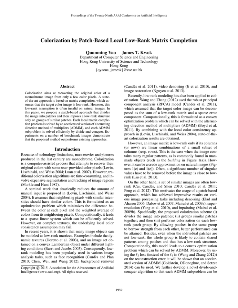
columns (resp. rows). This is the case when the image contains many regular patterns, as is commonly found in manmade objects (such as the building in Figure 1(a)). However, it can be a crude approximation on natural images (Figures 1(c) and 1(e)). Often, a significant number of singular
values have to be removed before the image is close to lowrank (Liu et al. 2013).
On the other hand, a set of similar images are often lowrank (Cai, Candès, and Shen 2010; Candès et al. 2011;
Peng et al. 2012). This motivates the usage of a patch-based
approach, which has achieved impressive results on various image processing tasks including denoising (Elad and
Aharon 2006; Dabov et al. 2007; Mairal et al. 2009a), superresolution (Yang et al. 2010), and inpainting (Mairal et al.
2009b). Specifically, the proposed colorization scheme (i)
divides the image into patches; (ii) groups similar patches
together; and then (iii) performs colorization on each lowrank patch group. By allowing patches in the same group
to borrow strength from each other, better performance can
be attained. Besides, even when the individual patches are
not low-rank, the whole group is likely to contain shared
patterns among patches and thus has a low-rank structure.
Computationally, this model leads to a convex optimization
problem which can be solved by ADMM. Moreover, by using the `2 loss (instead of the `1 in (Wang and Zhang 2012))
on the reconstruction error, it will be shown that an accelerated version of ADMM (Goldstein, ODonoghue, and Setzer
2014) can be used. We further develop a novel divide-andconquer algorithm so that each ADMM subproblem can be
Colorization aims at recovering the original color of a
monochrome image from only a few color pixels. A stateof-the-art approach is based on matrix completion, which assumes that the target color image is low-rank. However, this
low-rank assumption is often invalid on natural images. In
this paper, we propose a patch-based approach that divides
the image into patches and then imposes a low-rank structure
only on groups of similar patches. Each local matrix completion problem is solved by an accelerated version of alternating
direction method of multipliers (ADMM), and each ADMM
subproblem is solved efficiently by divide-and-conquer. Experiments on a number of benchmark images demonstrate
that the proposed method outperforms existing approaches.
Introduction
Because of technology limitations, most movies and pictures
produced in the last century are monochrome. Colorization
is a computer-assisted process that attempts to recover their
original colors with some user-provided color pixels (Levin,
Lischinski, and Weiss 2004; Luan et al. 2007). However, traditional colorization algorithms are time-consuming, and involve expensive segmentation and tracking of image regions
(Markle and Hunt 1987).
A seminal work that drastically reduces the amount of
manual input is proposed in (Levin, Lischinski, and Weiss
2004). It assumes that neighboring pixels with similar intensities should have similar colors. This is formulated as an
optimization problem which minimizes the difference between the color at each pixel and the weighted average of
colors from its neighboring pixels. Computationally, it leads
to a sparse linear system which can be efficiently solved.
However, on complex textures, the underlying local color
consistency assumption may fail.
In recent years, it is shown that many image objects can
be modeled as low-rank matrices. Examples include the dynamic textures (Doretto et al. 2003), and an image set obtained on a convex Lambertian object under different lighting conditions (Basri and Jacobs 2003). Consequently, lowrank modeling has been popularly used in various image
analysis tasks, such as face recognition (Candès and Plan
2010; Chen, Wei, and Wang 2012), background removal
c 2015, Association for the Advancement of Artificial
Copyright Intelligence (www.aaai.org). All rights reserved.
1959
(a) building.
(b) spectrum.
(c) castle.
(d) spectrum.
(e) lake.
(f) spectrum.
Figure 1: Singular value spectra of the building, castle and lake images.
or more separable blocks (Hong and Luo 2012)
solved efficiently.
The rest of this paper is organized as follows. We first provide short reviews on ADMM and RPCA. Next, we present
the proposed formulation (and the associated optimization
solver) based on patch-based low-rank matrix completion.
The last section provides experimental results on a number
of benchmark images and some concluding remarks.
Notations: In the sequel, the transpose of a vector / matrix
is denoted by the superscript (·)> , and the identity matrix
by I. Moreover, for a matrix A = [aij ] ∈ Rm×n , kAkF =
q
P
P
2
i,j aij is the Frobenius norm, kAk∗ =
i σi (where
σi ’s are the singular values of A) is the nuclear norm, and
vec(A) ∈ Rmn stacks the columns of A to a vector. Besides,
for two matrices A = [aij ], B = [bij ] ∈ Rm×n , A B =
m×n
[aij bij ] is the Hadamard
product. For A ∈
and B ∈

R
a11 B · · · a1n B


..
..
Rp×q , A⊗B = 
 is the Kronecker
.
.
am1 B · · · amn B
product. Finally, for a = [ai ] ∈ Rn , Diag(a) reshapes it to a
diagonal matrix with elements ai ’s.
min
x1 ,...,xK
In recent years, the alternating direction method of multipliers (ADMM) has been popularly used in diverse fields
such as machine learning, data mining and image processing (Boyd et al. 2011). Consider optimization problems of
the form
(1)
where φ, ψ are convex functions, and A, B (resp. c) are
constant matrices (resp. vector). ADMM considers the augmented Lagrangian L(x, y, ν) = φ(x) + ψ(y) + ν T (Ax +
By−c)+ ρ2 kAx+By−ck2 , where ν is the dual variable, and
ρ > 0 is a penalty parameter. At the tth iteration, the values
of x and y (denoted xt and yt ) are updated by minimizing
L(x, y, νt−1 ) w.r.t. x and y in an alternating manner:
xt
=
arg min L(x, yt−1 , νt−1 ),
yt
=
arg min L(xt , y, νt−1 ),
K
X
Ai xi = ci .
i=1
Algorithm 1 Accelerated ADMM (Goldstein, ODonoghue,
and Setzer 2014).
1: Initialize: y0 = ŷ1 = 0, ν0 = ν̂1 = 0, ρ > 0, α1 = 1,
and η ∈ (0, 1).
2: for t = 1, 2, . . . do
3:
xt = arg minx L(x, ŷt , ν̂t );
4:
yt = arg miny L(xt , y, ν̂t );
5:
νt = ν̂t + ρ (Axt + Byt − c);
2
2
6:
ct = ρ−1 kνt − ν̂t k + ρ kB(yt − ŷt )k ;
7:
if ct < ηct−1 thenp
8:
αt+1 = 12 (1 + 1 + 4αt2 );
−1
9:
ŷt+1 = yt + ααtt+1
(yt − yt−1 );
αt −1
10:
ν̂t+1 = νt + αt+1 (νt − νt−1 );
11:
else
12:
αt+1 = 1, ŷt+1 = yt , ν̂t+1 = νt ;
13:
ct = η −1 ct−1 ;
14:
end if
15: end for
Alternating Direction Method of Multipliers
x,y
i=1
φi (xi ) s.t.
A number of interesting ADMM applications with K ≥ 3
blocks can be found in (Ma 2012).
The standard ADMM algorithm above has a convergence
rate of O(1/T ), where T is the number of iterations (He
and Yuan 2012). Recently, inspired by the acceleration techniques for gradient descent methods (Beck and Teboulle
2009; Nesterov 2004), Goldstein, ODonoghue, and Setzer
(2014) proposed an accelerated version of ADMM (Algorithm 1), which has a much faster O(1/T 2 ) convergence
rate. However, this acceleration only works for the twoblock ADMM. Extension to multiple blocks is still open.
Related Works
min φ(x) + ψ(y) : Ax + By = c,
K
X
Robust Principal Component Analysis
Recently, Wang and Zhang (2012) proposed a state-of-theart colorization algorithm based on RPCA. Here, we consider RGB color images. Each m × n color image has three
color components (red, green and blue), and these together
can be represented by a matrix of size m × 3n.
Given a monochrome image G ∈ Rm×n , and a small
subset of user-provided color pixels (with values stored in
O ∈ Rm×3n , and their positions indicated by the binary matrix Ω ∈ {0, 1}m×3n ). The target color image L ∈ Rm×3n
x
y
and then ν is updated as νt = νt−1 + ρ(Axt + Byt − c).
While (1) has only two blocks of variables (x and y), the
ADMM has been recently extended to problems with three
1960
where T = [I, I, I] is a linear transform that averages
the three color components to form a monochrome image.
The first term in (2) measures the discrepancy between the
transformed and observed monochrome images; the second
term measures the difference with the observed color pixels;
while the last term encourages L to be low-rank. For efficient optimization, (2) is rewritten as
1
minL,X,E
kLT − Gk2F + λkΩ Ek1 + µkXk∗
2
s.t.
O = L + E, L = X,
(3)
patch at position (i, j) be Pi,j ∈ Rr×r . The similarity between patches Pi,j and Pi0 ,j 0 is defined
as kPi,j −
Pi0 ,j 0 k2F + β m12 (i − i0 )2 + n12 (j − j 0 )2 . The first term
measures similarity in terms of pixel intensity, while the last
two measure the physical distance. β is a trade-off parameter, and is set to 1 in the experiments.
For a given image patch, the standard block matching operation (Dabov et al. 2007) can be used to find its k most
similar patches in step 3. However, this takes O(kr2 D2 )
time (where D is the maximum search distance), and can
be expensive when D is large. In this paper, we perform the search more efficiently using approximate nearest neighbors (Muja and Lowe 2014). Its time complexity
is O(kr2 log N ), where N is the total number of patches.
Empirically, this is much faster than block matching.
which is then solved by ADMM. However, as there are three
variable blocks, the accelerated ADMM cannot be used.
Local Low-Rank Factorization
is obtained by the following optimization problem:
1
min kLT − Gk2F + λkΩ (L − O)k1 + µkLk∗ , (2)
L
2
>
For each image patch, let the k most similar patches (includ2
ing itself) be contained in the matrix G̃ ∈ Rr ×k . Similar to
(2), these patches can be colorized by solving the following
optimization problem
Proposed Algorithm
While a set of similar natural images can often be effectively
approximated by a low-rank matrix (Cai, Candès, and Shen
2010; Candès et al. 2011; Peng et al. 2012), Wang and Zhang
(2012) assumed that a single image (i.e., the target color image L) is low-rank. As discussed in the introduction, this
requires L to have regular patterns, which may not be valid
on natural images.
In this paper, instead of assuming that the whole L is lowrank, we first extract groups of similar image patches, and
then only assume that each group has a low-rank structure.
As will be seen, this group-based local low-rank assumption
is more appropriate and leads to better colorization performance. The proposed procedure, which will be called Patchbased Local Low-Rank colorization (PaLLR) in the sequel,
is shown in Algorithm 2. Note that in step 2, the uncolored
patches are selected as in BM3D (Dabov et al. 2007) (i.e.,
from top-left to bottom-right of the image). However, the
exact order is not important and preliminary results show
that random selection yields similar performance.
min
L̃
1
λ
kL̃T̃ − G̃k2F + kΩ̃ (L̃ − Õ)k2F + µkL̃k∗ , (4)
2
2
where Õ and Ω̃ indicate the values and positions of the
color pixels in these k patches, T̃ ∈ R3k×k is the color-to2
monochrome linear transform, and L̃ ∈ Rr ×3k is the target
colorization of G̃. While (2) assumes that the whole image is
low-rank, here this is assumed only on each group of similar
image patches. Figure 2(a) shows the singular value spectrum of a typical patch group. Compared to Figure 1(d), the
patch group has a much lower rank.
Algorithm 2 PaLLR procedure.
1: input: monochrome image; a small set of color pixels.
2: while there exists a patch P not yet colored do
3:
find k − 1 patches that are most similar to P ;
4:
obtain colorization for the group of k patches (by
solving (4) with accelerated ADMM in Algorithm 1);
5: end while
6: for each patch P do
7:
perform (weighted) average on the colorization results from all groups containing P ;
8: end for
9: for each pixel in the image do
10:
average the values from overlapping patches.
11: end for
(a) group of patches.
(b) one patch.
Figure 2: Singular value spectra on a patch group and single
patch (castle image).
Another difference with (2) is that the `2 loss, instead of
the `1 , is used on the low-rank reconstruction error. As will
be seen in the next section, this leads to a simpler optimization problem, with fewer optimization variables and allows
the use of accelerated ADMM.
Combining the Colorization Results
Since a patch may belong to multiple groups, its colorizations from different groups can be different. These can be
combined by weighted averaging, with smaller contributions
from the more distant groups. Finally, one has to assemble
the whole image from the overlapping colorized patches. As
is common in patch-based image processing (Dabov et al.
Grouping of Similar Image Patches
Given a monochrome image (of size m × n), we first
extract overlapping patches each of size r × r. Let the
1961
2007), the color of a pixel is obtained by averaging the color
values in patches containing it.
Algorithm 3 FastInv(M ): Fast inverse on a sub-matrix M
of R using divide-and-conquer.
1: if M is of size k × k then
2:
invert M using (7);
3: else
4:
partition
M to 4 equal-sized sub-matrices
M11 M12
;
M21 M22
−1
5:
M22
= FastInv(M22 );
−1
−1
6:
U ="FastInv(M11 − M12 M22
M21 );
#
Solving (4) Using Accelerated ADMM
In this section, we discuss how to efficiently solve the local
low-rank factorization problem in (4). First, we rewrite it as
1
λ
minL̃,X kL̃T̃ − G̃k2F + kΩ̃ (L̃ − Õ)k2F + µkXk∗
2
2
s.t. X = L̃.
(5)
Since we only have two variable blocks, it can be readily
solved using the accelerated ADMM algorithm. The first
two terms in the objective of (5) together play the role of
φ, and the last term is ψ. The augmented Lagrangian is
L(L̃, X, Q) = 12 kL̃T̃ − G̃k2F + λ2 kΩ̃(L̃− Õ)k2F +µkXk∗ +
tr(Q> (L̃ − X)) + ρ2 kL̃ − Xk2F , where Q is the dual variable.
Thus, in Algorithm 1, variable x becomes L̃, y becomes X,
and ν becomes Q. The two core steps are the updates of L̃
and X, which will be discussed in the following.
7:
M −1 =
U −1
−1
−M22
M21 U −1
−1
−U −1 M12 M22
−1
−1
−1 .
M22
+ M22
M21 U −1 M12 M22
8: end if
It can be easily seen that R−1 , like R, is also sparse and
has only O(m̃ñ) nonzero elements. Thus, on recovering L̃t
from (6) (as vec(L̃t ) = R−1 vec(C)), this matrix-vector
multiplication takes O(m̃ñ) time. In total, the L̃ update takes
O(m̃ñ log m̃) time, which is much faster than both direct
matrix inversion and conjugate gradient.
ADMM Update on L̃
Step 2 in Algorithm 1 becomes minL̃ 12 kL̃T̃ − G̃k2F +
2
ρ
λ 2
Ω̃
(
L̃
−
Õ)
+ tr(Q̂>
t (L̃ − X̂t )) + 2 kL̃ − X̂t kF . Set2
ADMM Update on X
Step 3 in Algorithm 1 can be rewritten as:
2
1
1
+ µ kXk∗ .
Xt = arg min X
−
L̃
+
Q̂
t
t
X 2
ρ
ρ
F
F
ting its derivative w.r.t. L̃ to zero, and using properties of the
Hadamard and Kronecker products, it is easy to see that L̃t
can be obtained as
R vec L̃t = vec(C),
(6)
where R = T̃ T̃ > ⊗ I + λDiag vec Ω̃
+ ρI, and
C = G̃T̃ > + λ Ω̃ Õ + ρX̂t − Q̂t . This is a simple
It is well-known that this reduces to the singular
value
1
thresholding (SVT) operator SVT µρ L̃t + ρ Q̂t (Cai,
Candès, and Shen 2010). In general, let U ΣV > be the SVD
of a matrix Z. Then, SVTτ (Z) = U (Σ − τ I)+ V > . The
SVT operation here takes O (m̃ñ min(m̃, ñ)) time.
linear system. However, as R ∈ Rm̃ñ×m̃ñ (where, for simplicity of notations, we denote m̃ = r2 and ñ = 3k), a
naive matrix inversion takes O(m̃3 ñ3 ) time. Alternatively,
iterative approaches such as conjugate gradient (CG) can be
used. Empirically, this is faster, though each CG iteration
takes O(m̃ñ) time and O(min(m̃, ñ)) iterations are required
for convergence (Nocedal and Wright 2006).
Much faster matrix inversion is possible by exploiting the
structure of R. Observe that R can be partitioned into (3r2 )2
blocks (each of size k × k), with the (i, j)th block being
I
i 6= j
ij
B =
,
λDiag(ωi ) + (1 + ρ)I i = j
Discussion
Recall that if kΩ̃ (L̃ − Õ)k2F in (4) is replaced by kΩ̃ (L̃ − Õ)k1 , the optimization problem will be of the same
form as (2) and the solver in (Wang and Zhang 2012) can be
used. While the per-iteration complexity in both solvers are
dominated by the SVT step, (3) involves three primal and
two dual variables, but (5) only has two primal variables and
one dual variable. Hence, ours is faster by a constant factor.
More importantly, since (5) has only two variable blocks, the
accelerated ADMM can be used, while (3) can only use the
standard ADMM. As shown in (Goldstein, ODonoghue, and
Setzer 2014), the difference in convergence rates (namely,
O(1/T 2 ) vs O(1/T )) can lead to a significant difference in
the number of iterations required.
The proposed PaLLR algorithm is related to the recent local low-rank matrix approximation (LLORMA) algorithm (Lee et al. 2013; 2014), which has demonstrated
encouraging results on recommendation systems. However,
LLORMA may not be appropriate for colorization. When
used in this context, it assumes that all image patches are
low-rank (Table 1). For each patch, a low-rank matrix completion problem (similar to (2) and (4)) is solved. However,
and ωi is the sub-vector in vec(Ω̃) containing its (ik 2 + 1)th
−1
to (i + 1)k 2 th elements. As B ij is diagonal, B ij
can be
easily obtained in O(k) time as
−1
I
i 6= j
B ij
=
. (7)
Diag (1./ (λωi + (1 + ρ)1)) i = j
Here, we use the MATLAB notation and the ./ operator performs division on each element of the vector separately. Using divide-and-conquer and the equation for partitioned matrix inverse, R−1 can be efficiently obtained as FastInv(R)
using Algorithm 3 in O(m̃ñ log m̃) time.
1962
method
(Wang and Zhang 2012)
(Lee et al. 2013)
proposed method
entity of low-rank structure
whole image
each single patch
group of similar patches
Table 1: Low-rank assumptions used by various methods.
an image patch is small, and thus unlikely to contain repetitive patterns or regular structures at such a scale. Consequently, its rank may not be low (Figure 2(b)). As will be
seen from the experimental results, this low-rank assumption leads to inferior colorization performance.
One potential problem with local algorithms (such as the
proposed PaLLR and LLORMA) is that a large number of
local models may have to be learned. To alleviate this problem, instead of computing a local model at each possible location, LLORMA only randomly chooses a subset as anchor
points for the local models. For PaLLR, we only learn colorizations for patches that have not yet been colorized. As
each group has k patches, this reduces the number of local
models by about k times. Moreover, the optimization variables in (4) are much smaller than those in (2) (m̃ñ vs mn).
Besides, as in LLORMA, local low-rank factorizations for
multiple image patches can be easily parallelized.
(a) castle.
Experiments
Experiments are performed on eight color images from the
Berkeley segmentation data set (Figure 3). These have also
been used in (Wang and Zhang 2012), and we follow the
same setup. For each color image, the monochrome version
is obtained by averaging the R, G and B components. Varying numbers of pixels (1% − 10%) are randomly sampled
from the color image as observed labels input to the colorization algorithm. The following methods will be compared:1
(c) mushroom.
(d) woman.
(e) couple.
(f) lake.
(g) landscape.
(h) street.
Figure 3: Images used in the experiments. (a)-(d) are of size
481 × 321, (e)-(h) are of size 321 × 481.
PaLLR operate on image patches. We fix the patch size r to
16, and use k = 50 patches in each PaLLR group. As will be
seen, the performance is again not sensitive to these settings.
In (Lee et al. 2013; 2014), the local models of LLORMA
are positioned at random locations. To avoid the possible
statistical variation, here we construct its local models at
all patches. Hence, LLORMA has an unfair advantage over
PaLLR as it uses more local models.
For performance evaluation, we use the peak signal-tonoise ratio (PSNR) which has been commonly used in image processing (Elad and Aharon 2006). Let the original
color image be I˜ ∈ Rm×3n and the colorization result be
Iˆ ∈ Rm×3n , PSNR is defined as 10 log10 255
∆ , where
qP
P
3n
m
(I˜ij − Iˆij )2 .
∆= 1
1. Local color consistency (LCC) (Levin, Lischinski, and
Weiss 2004);
2. Global low-rank matrix completion (GLR) (Wang and
Zhang 2012): The values of λ and µ are set as suggested
in (Wang and Zhang 2012);
3. Local low-rank matrix approximation (LLORMA) (Lee
et al. 2013): To be consistent with PaLLR, each local matrix factorization is based on (4), and the resultant local
colorization results are combined as in PaLLR.
4. The proposed PaLLR: We experiment with both `1 and
`2 losses for the reconstruction error. For `1 , we follow
the parameter setting in GLR. For `2 , note that the first
term in (4) sums over r2 k pixels, while the second term
sums over nΩ̃ pixels (where nΩ̃ is the number of 1’s in
Ω̃). Thus, we set λ ∝ r2 k/nΩ̃ . In the experiments, we fix
the proportionality constant to 5, and µ = 0.16. As will
be seen, the performance is not sensitive to these settings.
3mn
i=1
j=1
Results
Results on PSNR are shown in Figure 4. As can be seen,
PaLLR significantly outperforms the other methods, and the
improvement increases with the number of labeled color pixels. Using `1 or `2 for the reconstruction error in PaLLR lead
to very similar PSNR results, but using `2 is about 4 times
faster. Overall, GLR outperforms LCC (except on the images street and woman) and is in the second place in terms
of PSNR. LLORMA is the worst, even though it uses more
patches and thus more local models.
Colorization results and difference images are shown in
Figures 5 and 6, respectively. The LLORMA results are in-
As suggested by (Wang and Zhang 2012), local color
consistency is used as preprocessing for GLR, LLORMA,
and PaLLR. This expands the initial set of color pixels,
and makes colorization easier. Besides, both LLORMA and
1
(b) koala.
Codes for LCC and GLR are obtained from their authors.
1963
(a) castle.
(b) couple.
(c) koala.
(d) lake.
(e) landscape.
(f) mushroom.
(g) street.
(h) woman.
Figure 4: PSNR results on the various images.
For GLR, artifacts can be seen. Moreover, while the errors
produced by GLR and PaLLR are localized, those by LCC
are more diffused.
Finally, we study the effects on varying the patch size r,
group size r and regularization parameters (µ and λ) in (4).
As can be seen from Figure 7, PaLLR is stable over a wide
range of parameter settings.
(a) LCC.
(e) LCC.
(b) GLR.
(f) GLR.
(c) LLORMA.
(g) LLORMA.
(d) PaLLR.
(a) patch size.
(b) group size.
(c) µ.
(d) λ.
(h) PaLLR.
Figure 5: Colorization results on castle (1% labels) and
woman (10% labels). Artifacts for GLR are circled in red.
Figure 7: Variation in PSNR with different parameter settings on the castle image.
ferior, which agree with the previous observations on PSNR.
Conclusion
(a) LCC.
(b) GLR.
(c) LLORMA.
In this paper, we extended the matrix completion approach
for colorization. Instead of using a low-rank structure on
the whole image, we adopted a patch-based scheme and imposed this assumption only on each group of similar patches.
The resultant optimization problem can be solved by accelerated ADMM, with the ADMM subproblem efficiently
solved with a novel divide-and-conquer algorithm. Experimental results demonstrate that the proposed method outperforms existing approaches.
(d) PaLLR.
Figure 6: Differences between the original castle image and
various colorization results in Figure 5.
1964
Acknowledgments
Lee, J.; Bengio, S.; Kim, S.; Lebanon, G.; and Singer, Y.
2014. Local collaborative ranking. In Proceedings of the
23rd International Conference on World Wide Web, 85–96.
Levin, A.; Lischinski, D.; and Weiss, Y. 2004. Colorization using optimization. ACM Transactions on Graphics
23(3):689–694.
Liu, J.; Musialski, P.; Wonka, P.; and Ye, J. 2013. Tensor completion for estimating missing values in visual data.
IEEE Transactions on Pattern Analysis and Machine Intelligence 35(1):208–220.
Luan, Q.; Wen, F.; Cohen-Or, D.; Liang, L.; Xu, Y.-Q.; and
Shum, H.-Y. 2007. Natural image colorization. In Proceedings of the 18th Eurographics conference on Rendering
Techniques, 309–320.
Ma, S. 2012. Alternating proximal gradient method for convex minimization. Technical report.
Mairal, J.; Bach, F.; Ponce, J.; Sapiro, G.; and Zisserman, A.
2009a. Non-local sparse models for image restoration. In
Proceedings of the 12th International Conference on Computer Vision, 2272–2279.
Mairal, J.; Bach, F.; Ponce, J.; and Sapiro, G. 2009b. Online
dictionary learning for sparse coding. In Proceedings of the
26th International Conference on Machine Learning, 689–
696.
Markle, W., and Hunt, B. 1987. Coloring a black and white
signal using motion detection. Patent US4755870 A.
Muja, M., and Lowe, D. 2014. Scalable nearest neighbour
algorithms for high dimensional data. IEEE Transactions on
Pattern Analysis and Machine Intelligence.
Nesterov, Y. 2004. Introductory Lectures on Convex Optimization: A Basic Course. Springer.
Nguyen, H.; Peng, X.; Do, M.; and Liang, Z.-P. 2013. Denoising MR spectroscopic imaging data with low-rank approximations. IEEE Transactions on Biomedical Engineering 60(1):78–89.
Nocedal, J., and Wright, S. J. 2006. Numerical Optimization. Springer.
Peng, Y.; Ganesh, A.; Wright, J.; Xu, W.; and Ma, Y. 2012.
RASL: Robust alignment by sparse and low-rank decomposition for linearly correlated images. IEEE Transactions
on Pattern Analysis and Machine Intelligence 34(11):2233–
2246.
Wang, S., and Zhang, Z. 2012. Colorization by matrix completion. In Proceedings of the 26th Conference on Artificial
Intelligence.
Yang, J.; Wright, J.; Huang, T. S.; and Ma, Y. 2010. Image
super-resolution via sparse representation. IEEE Transactions on Image Processing 19(11):2861–2873.
This research was supported in part by the Research Grants
Council of the Hong Kong Special Administrative Region
(Grant 614513).
References
Basri, R., and Jacobs, D. W. 2003. Lambertian reflectance
and linear subspaces. IEEE Transactions on Pattern Analysis and Machine Intelligence 25(2):218–233.
Beck, A., and Teboulle, M. 2009. A fast iterative shrinkagethresholding algorithm for linear inverse problems. SIAM
Journal on Imaging Sciences 2(1):183–202.
Boyd, S.; Parikh, N.; Chu, E.; Peleato, B.; and Eckstein, J.
2011. Distributed optimization and statistical learning via
the alternating direction method of multipliers. Foundations
and Trends of Machine Learning 3(1):1–122.
Cai, J.; Candès, E. J.; and Shen, Z. 2010. A singular value
thresholding algorithm for matrix completion. SIAM Journal on Optimization 20:1956–1982.
Candès, E. J., and Plan, Y. 2010. Matrix completion with
noise. Proceedings of the IEEE 98(6):925–936.
Candès, E. J.; Li, X.; Ma, Y.; and Wright, J. 2011. Robust
principal component analysis. Journal of the ACM 58(3):1–
37.
Chen, C.-F.; Wei, C.-P.; and Wang, Y.-C. F. 2012. Low-rank
matrix recovery with structural incoherence for robust face
recognition. In Proceedings of the International Conference
on Computer Vision and Pattern Recognition, 2618–2625.
Dabov, K.; Foi, A.; Katkovnik, V.; and Egiazarian, K. 2007.
Image denoising by sparse 3-D transform-domain collaborative filtering. IEEE Transactions on Image Processing
16(8):2080–2095.
Doretto, G.; Chiuso, A.; Wu, Y.; and Soatto, S. 2003. Dynamic textures. International Journal of Computer Vision
51(2):91–109.
Elad, M., and Aharon, M. 2006. Image denoising via
sparse and redundant representations over learned dictionaries. IEEE Transactions on Image Processing 15(12):3736–
3745.
Goldstein, T.; ODonoghue, B.; and Setzer, S. 2014. Fast
alternating direction optimization methods. SIAM Journal
on Imaging Sciences 7(3).
He, B., and Yuan, X. 2012. On the O(1/n) convergence
rate of the Douglas-Rachford alternating direction method.
SIAM Journal on Numerical Analysis 50(2):700–709.
Hong, M., and Luo, Z.-Q. 2012. On the linear convergence
of the alternating direction method of multipliers. Technical
Report arXiv:1208.3922.
Ji, H.; Liu, C.; Shen, Z.; and Xu, Y. 2010. Robust video denoising using low rank matrix completion. In Proceedings of
the International Conference on Computer Vision and Pattern Recognition, 1791–1798.
Lee, J.; Kim, S.; Lebanon, G.; and Singer, Y. 2013. Local
low-rank matrix approximation. In Proceedings of the 30th
International Conference on Machine Learning, 82–90.
1965