Proceedings of the Thirtieth AAAI Conference on Artificial Intelligence (AAAI-16)
Randomised Procedures for Initialising and Switching Actions in Policy Iteration
Shivaram Kalyanakrishnan
Indian Institute of Technology Bombay
Mumbai 400076 India
shivaram@cse.iitb.ac.in
Neeldhara Misra
Aditya Gopalan
Indian Institute of Technology Gandhinagar
Gandhinagar 382355 India
neeldhara.misra@gmail.com
Indian Institute of Science
Bengaluru 560012 India
aditya@ece.iisc.ernet.in
to act. This problem, referred to as MDP planning, is the
focus of this paper.
Formally, an MDP M “ pS, A, R, T, γq has a set of states
S in which an agent can be, and a set of actions A that the
agent can execute. Upon taking action a from state s, the
agent receives a reward r, assumed to be a real-valued random variable with mean Rps, aq. The action a also transports the agent to a state s1 , selected from S at random with
probability T ps, a, s1 q. In this paper, we assume that S and
A are both finite, with |S| “ n ě 2, and |A| “ k ě 2.
To fully specify M , we need to define an objective for
the agent. A policy (assumed stationary, deterministic, and
Markovian) is a mapping from S to A: when following
a policy π, the agent takes action πpsq when in state s.
A natural objective is to find a policy that maximises the
agent’s expected long-term reward. Consider an agent that
starts in some state s0 at time 0 and continually follows
π. The agent thereby encounters a trajectory over time:
xs0 , πps0 q, r0 , s1 , πps1 q, r1 , s2 , . . . y. The value of state s
under policy π is given by
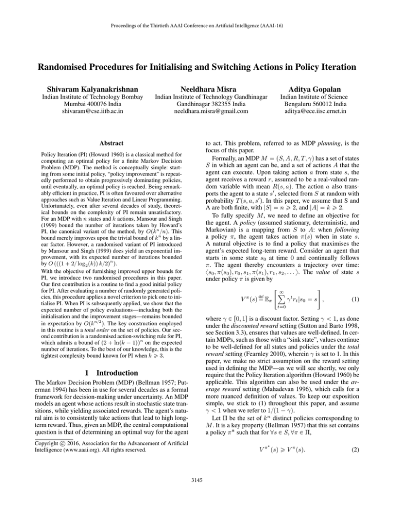
ff
«
8
ÿ
def
γ t rt |s0 “ s ,
(1)
V π psq “ Eπ
Abstract
Policy Iteration (PI) (Howard 1960) is a classical method for
computing an optimal policy for a finite Markov Decision
Problem (MDP). The method is conceptually simple: starting from some initial policy, “policy improvement” is repeatedly performed to obtain progressively dominating policies,
until eventually, an optimal policy is reached. Being remarkably efficient in practice, PI is often favoured over alternative
approaches such as Value Iteration and Linear Programming.
Unfortunately, even after several decades of study, theoretical bounds on the complexity of PI remain unsatisfactory.
For an MDP with n states and k actions, Mansour and Singh
(1999) bound the number of iterations taken by Howard’s
PI, the canonical variant of the method, by Opkn {nq. This
bound merely improves upon the trivial bound of kn by a linear factor. However, a randomised variant of PI introduced
by Mansour and Singh (1999) does yield an exponential improvement, with its expected number of iterations bounded
by O ppp1 ` 2{ log2 pkqq k{2qn q.
With the objective of furnishing improved upper bounds for
PI, we introduce two randomised procedures in this paper.
Our first contribution is a routine to find a good initial policy
for PI. After evaluating a number of randomly generated policies, this procedure applies a novel criterion to pick one to initialise PI. When PI is subsequently applied, we show that the
expected number of policy evaluations—including both the
initialisation and the improvement stages—remains bounded
in expectation by Opkn{2 q. The key construction employed
in this routine is a total order on the set of policies. Our second contribution is a randomised action-switching rule for PI,
which admits a bound of p2 ` lnpk ´ 1qqn on the expected
number of iterations. To the best of our knowledge, this is the
tightest complexity bound known for PI when k ě 3.
t“0
The Markov Decision Problem (MDP) (Bellman 1957; Puterman 1994) has been in use for several decades as a formal
framework for decision-making under uncertainty. An MDP
models an agent whose actions result in stochastic state transitions, while yielding associated rewards. The agent’s natural aim is to consistently take actions that lead to high longterm reward. Thus, given an MDP, the central computational
question is that of determining an optimal way for the agent
where γ P r0, 1s is a discount factor. Setting γ ă 1, as done
under the discounted reward setting (Sutton and Barto 1998,
see Section 3.3), ensures that values are well-defined. In certain MDPs, such as those with a “sink state”, values continue
to be well-defined for all states and policies under the total
reward setting (Fearnley 2010), wherein γ is set to 1. In this
paper, we make no strict assumption on the reward setting
used in defining the MDP—as we will see shortly, we only
require that the Policy Iteration algorithm (Howard 1960) be
applicable. This algorithm can also be used under the average reward setting (Mahadevan 1996), which calls for a
more nuanced definition of values. To keep our exposition
simple, we stick to (1) throughout this paper, and assume
γ ă 1 when we refer to 1{p1 ´ γq.
Let Π be the set of k n distinct policies corresponding to
M . It is a key property (Bellman 1957) that this set contains
a policy π ˚ such that for @s P S, @π P Π,
c 2016, Association for the Advancement of Artificial
Copyright Intelligence (www.aaai.org). All rights reserved.
V π psq ě V π psq.
1
Introduction
‹
3145
(2)
Such a policy π ‹ is called an optimal policy (in general there
could be multiple optimal policies for an MDP).
The problem we consider is precisely that of finding an
optimal policy for a given MDP M “ pS, A, R, T, γq.1
Specifically, we examine the Policy Iteration (PI) (Howard
1960) family of algorithms, which follow the general template of starting with some initial policy, and repeatedly
computing local improvements until an optimal policy is
found. In most MDPs encountered in practice, the number of such improvements (or “iterations”) needed to find
an optimal policy is relatively small compared to the size
of the MDP. However, there do exist MDPs wherein PI
may be forced to pass through lengthy improvement sequences (Fearnley 2010). From a theoretical standpoint, it
has proven hard to establish tight upper bounds on the number of iterations taken by PI: the best existing upper bounds
are of the form Oppk{2qn q, when k is large, for a randomised
variant of PI proposed by Mansour and Singh (1999). Indeed
the aim of this paper is to provide better formal guarantees.
To this end, we propose two algorithms.
1. Our first contribution is a randomised procedure titled
“Guess-and-Max”, which picks a good initial policy for
PI. We show that regardless of the PI algorithm subsequently applied, the total number of policy evaluations
remains bounded by Opk n{2 q in expectation..
2. Our second contribution is a randomised improvement
operator for a variant of PI called “Simple” PI (Melekopoglou and Condon 1994). We bound the expected number of iterations in the resulting algorithm, which we call
Randomised Simple PI (RSPI), by p2 ` lnpk ´ 1qqn .
This paper is organised as follows. In Section 2, we give
an overview of approaches for MDP planning, and therein
highlight the appeal of PI, which we describe in detail. In
sections 3 and 4, we present our two algorithms and the
corresponding analyses. We summarise our results and conclude the paper in Section 5.
2
Qπ ps, aq denotes the expected long-term reward obtained
when the agent executes action a at state s once, and thereafter executes π. The value function corresponding to an optimal policy π ‹ is termed the optimal value function, denoted
V ‹ . Indeed V ‹ is the unique solution of another set of equations called Bellman’s Optimality Equations: @s P S,
˜
‹
V psq “ max Rps, aq ` γ
aPA
ÿ
¸
1
‹
1
T ps, a, s qV ps q .
s1 PS
V ‹ , Q‹ and π ‹ are easy to derive from each other. If V ‹ is
‹
known, it directly yields Q‹ “ Qπ , from which π ‹ can be
readily obtained: @s P S, π ‹ psq “ argmaxaPA Q‹ ps, aq. If
we start with π ‹ , then policy evaluation yields V ‹ , which, in
turn, gives Q‹ .
Owing to the presence of the max operator, solving Bellman’s Optimality Equations is not as straightforward as policy evaluation. Consequently, numerous planning algorithms
have been proposed in the literature. These algorithms can
be placed in the following broad categories.
2.1
Linear Programming (LP)
‹
V and π ‹ can be obtained by solving a linear program
based on Bellman’s Optimality Equations; typical formulations either involve n variables and nk constraints, or nk
variables and n constraints (Littman, Dean, and Kaelbling
1995, see Section 4.1). Assuming that exact floating point
arithmetic operations can be performed in unit time, algorithms such as the Interior-Point (Karmarkar 1984) and
Ellipsoid (Khachiyan 1980) methods for LP yield weakly
polynomial bounds on the running time. The corresponding
bounds are polynomial in n, k, and the number of bits B
needed to represent the MDP. The dependence on B arises
because these methods seek increasingly better approximations of the optimal solution, and this quest naturally gets
curtailed by machine precision.
A contrasting approach, which eliminates the dependence
on B, involves searching over a discrete set of solutions
that is known to contain the optimal one. Thus, by applying the Simplex method (Dantzig 1963) on the linear program resulting from an MDP, bounds can be obtained solely
in terms of n and k. While bounds for the canonical Simplex algorithm are in general exponential in n, it has been
shown that the method is strongly polynomial for deterministic MDPs (Post and Ye 2013). The best strong bounds
for LP are subexponential ones arising from randomised
vertex-switching methods (Kalai 1992; Matoušek, Sharir,
and Welzl 1996): the
? best that apply to general MDPs are
Oppolypn, kq expp2 nqq (Gärtner 2002).
Planning Algorithms and their Complexity
ÿ
T ps, πpsq, s1 qV π ps1 q.
s1 PS
In this section, we introduce some basic results pertaining to
MDPs before considering algorithms that build upon these
results. First, observe from (1) that the value function V π of
a policy π, which yields values at each state, can be specified
recursively: @s P S,
V π psq “ Rps, πpsqq ` γ
ÿ
Qπ ps, aq “ Rps, aq ` γ
T ps, πpsq, s1 qV π ps1 q.
s1 PS
This definition implies that the value function of a policy can be computed efficiently by solving a system of
n linear equations, which are called Bellman’s Equations.
Clearly this operation—called policy evaluation—requires
no more than Opn3 q arithmetic operations. With an additional Opn2 kq operations, the action value function function Qπ corresponding to policy π can be obtained from V π :
@s P S, @a P A,
2.2
Value Iteration (VI)
Although attractive in theory, LP-based methods seldom
perform better in practice when compared to “dynamic programming” techniques that compute V ‹ and π ‹ based on an
1
Thus, we need to solve a planning problem. In the related problem of learning (Sutton and Barto 1998), R and T are unknown,
but can be queried for samples of rewards and next states.
3146
iterated sequence. Starting with V 0 , an arbitrary initial guess
of V ‹ , the Value Iteration (VI) algorithm (Szepesvári 2010,
see Section 2.4) applies the following iteration. @s P S,
˜
V t`1 psq Ð max Rps, aq ` γ
aPA
ÿ
Theorem 2 (Policy improvement (Szepesvári 2010; Bertsekas 2012)). Let π, π 1 P Π be such that ISpπq ‰ H, and
π 1 satisfies (3). Then
¸
π 1 ą π.
T ps, a, s1 qV t ps1 q .
Proof. For convenience, we provide a proof of this “policy
improvement theorem”, which is standard material in textbooks on MDPs (Szepesvári 2010; Bertsekas 2012). The
main tool employed in the proof is the “Bellman Operator”
B π : pS Ñ Rq Ñ pS Ñ Rq, given by: @s P S,
ÿ`
˘
def
pB π pXqqpsq “
Rps, πpsqq ` γT ps, πpsq, s1 qXps1 q .
s1 PS
The “Bellman Optimality Operator” applied above is a
contraction in the max-norm, and Banach’s Fixed Point Theorem ensures that the sequence xV 0 , V 1 , V 2 , . . . y converges
to V ‹ (Szepesvári 2010, see Appendix A). The number of iterations to convergence is bounded by a polynomial in n, k,
1{p1´γq, and B (Littman, Dean, and Kaelbling 1995). Some
relatively simple changes to the update operator and the sequence of state-updates can speed up VI in practice (Sutton
and Barto 1998, see Section 9.4), but the inherent dependence on 1{p1 ´ γq implies unbounded growth as γ Ñ 1.
2.3
s1 PS
A moment’s reflection assures us that π 1 satisfying (3) is
equivalent to the following statement.
1
B π pV π q ą V π .
Now, it is easy to verify that for X : S Ñ R and Y : S Ñ R,
1
1
1
if X ľ Y , then B π pXq ľ B π pY q. Thus, applying B π to
1
1
both sides of (4), we get pB π q2 pV π q ľ B π pV π q. Applying
1
B π to both sides again and applying the transitivity of ľ ad
infinitum, we obtain:
Policy Iteration (PI)
We now consider the basis for Policy Iteration (PI), which is
the subject of this paper. For a given policy π, let ISpπq be
the set of states s on which π is not greedy with respect to
its own action value function: in other words,
"
π
def
π
(4)
*
ISpπq “ s P S : Q ps, πpsqq ă max Q ps, aq .
1
1
lim pB π ql pV π q ľ B π pV π q.
aPA
lÑ8
PI (Howard 1960) is an elegant approach based on the
observation that
1. If ISpπq ‰ H, then π can be “improved” by switching to
more promising actions on states in ISpπq;
2. If ISpπq “ H, then π is optimal.
Thus, ISpπq is the set of (locally) “improvable states” in π.
Specifically, for each state s in ISpπq, let IApπ, sq be the set
of actions that improve upon the action taken by π: that is,
It is well known that by Banach’s Fixed Point theorem , the
1
limit on the left evaluates to V π . Combining the above relation with (4) completes the proof.
Corollary 3 (Policy optimality). For π P Π, if ISpπq “ H,
then π is optimal.
Proof. Again we argue using the Bellman Operator:
1
ISpπq “ H ùñ @π 1 P Π : V π ľ B π pV π q
IApπ, sq “ ta P A : Qπ ps, aq ą V π psqu .
Now, assuming π is not optimal, let π 1 be a policy that in
one or more states s in ISpπq, takes an action belonging to
IApπ, sq, and in the remaining states, takes the same actions
as π: that is,
def
1
ùñ @π 1 P Π : V π ľ lim pB π ql pV π q
lÑ8
1
ðñ @π 1 P Π : V π ľ V π .
Indeed the PI algorithm essentially puts these results to
practice: starting with some initial policy, it repeatedly applies policy improvement until an optimal policy is reached.
Note that given a policy π, ISpπq and IApπ, ¨q can be obtained in Opn3 ` n2 kq time. Thus, the complexity of PI is
essentially determined by the number of iterations needed
to reach an optimal policy. Since the algorithm can visit no
policy twice (owing to strict improvement), the number of
iterations is trivially bounded by k n .
The elegant structure of PI facilitates complexity bounds
that are independent of B and γ, thereby contributing to the
method’s theoretical appeal.2 The key design choice within
PI is in the implementation of the improvement operator.
Theorem 2 holds for every choice of π 1 where some nonempty subset of ISpπq is “switched”, and for each state s
that is thereby chosen for switching, π 1 can adopt any from
Ds P S : π 1 psq P IApπ, sq, and
@s P S : pπ 1 psq “ πpsqq _ pπ 1 psq P IApπ, sqq.
(3)
It can be shown that π 1 improves upon (or dominates) π in
the following sense.
Definition 1 (ľ, ą). For functions X : S Ñ R, Y : S Ñ R,
we define X ľ Y if and only if
@s P S : Xpsq ě Y psq,
and we define X ą Y if and only if
X ľ Y and Ds P S : Xpsq ą Y psq.
For policies π1 , π2 P Π, we define π1 ľ π2 if and only if
V π1 ľ V π2 ,
and we define π1 ą π2 if and only if
V π1 ą V π2 .
2
Polynomial bounds involving 1{p1 ´ γq have also been shown
for PI (Ye 2011; Scherrer 2013).
3147
Let L be an arbitrary total order on Π, which we shall use
for tie-breaking. (For example, L could be taken as the lexicographic ordering of the set of all words of length n over
the alphabet A, each word representing a policy.)
For π1 , π2 P Π, we define π1 Ï π2 if and only if
action IApπ, sq. Which non-empty subset of ISpπq must we
choose, and to which actions must we switch? Does our
choice facilitate a tighter bound on the number of iterations?
In the canonical variant of PI (called Howard’s
PI) (Howard 1960), all switchable actions are switched in
every iteration: that is, the subset chosen for switching is
ISpπq itself. Thus, Howard’s PI implements a greedy variant of policy improvement, and is sometimes referred to
as Greedy PI. Mansour and Singh (1999) show that regardless of the strategy used for picking improving actions,
Howard’s PI requires at most 13k n {n iterations. Hollanders
et al. (2014) tighten this bound to pk{pk ´ 1q ` op1qqpk n {nq.
Mansour and Singh (1999) also propose a randomised
version of PI in which the subset of states to be improved is chosen uniformly at random from among the
non-empty subsets of ISpπq. For this algorithm, they show
that the expected number of iterations is bounded by
n
O ppp1 ` 2{ log2 pkqq k{2q q; again, the bound holds for every choice of action-switching rule. A tighter bound of
20.78n holds for k “ 2. In this case, there is at most one
improving action per state, and so no choice in switching.
Fearnley (2010) provides an MDP construction and an initial policy that takes Howard’s PI through Ωp2n{7 q iterations.
While Fearnley’s construction is for the total and average reward models, it has subsequently also been extended to the
discounted reward model (Hollanders, Gerencsér, and Delvenne 2012). These recent lower bounds for Howard’s PI
follow several years after Melekopoglou and Condon (1994)
showed a lower bound of Ωp2n{2 q for Simple PI, a variant in
which the improvable state with the highest index (assuming
a fixed indexing over S) is chosen for improvement. This
lower bound is shown on a two-action MDP.
Interestingly, we show a positive result based on Simple PI: faced with choice in action-switching (that is, when
k ě 3), we argue that it is efficient to choose an action uniformly at random from the improving set. To the best of our
knowledge, the corresponding bound of p2 ` lnpk ´ 1qqn expected iterations is the tightest complexity bound known for
the PI family of algorithms when k ě 3. Before describing
this result in Section 4, we present an approach that can be
coupled with any variant of PI to obtain an expected complexity bound of Oppolypn, kqk n{2 q for MDP planning.
3
V pπ1 q ą V pπ2 q, or
V pπ1 q “ V pπ2 q and π1 Lπ2 .
Observe that since L is a total order, so is Ï: that is,
1. @π1 , π2 P Π : π1 Ï π2 and π2 Ï π1 ùñ π1 “ π2 ;
2. @π1 , π2 , π3 P Π : π1 Ï π2 and π2 Ï π3 ùñ π1 Ï π3 ;
3. @π1 , π2 P Π : π1 Ï π2 or π2 Ï π1 .
Since Ï is a total order, we find it convenient to associate
a unique index with each policy π to denote the number of
policies it dominates under Ï:
ˇ
ˇ
π def ˇ
IÏ
“ tπ 1 P Π : π Ï π 1 uˇ .
Clearly this index ranges from 1 to |Π|, with the highest index belonging to an optimal policy. Note that @π, π 1 P Π :
π
π1
π
ě IÏ
ðñ π Ï π 1 . Hereafter, we refer to IÏ
as the
IÏ
“Ï-index” of π.
Given any two policies, observe that they can be compared under Ï with just two policy evaluations (in Opn3 q
time). More crucially, observe that Ï is designed to be “respected” by ą, and consequently by policy improvement.
Lemma 5 (Policy improvement respects Ï). For π, π 1 P Π,
if policy improvement to π yields π 1 , then π 1 Ï π.
Proof. Since policy improvement to π yields π 1 , it follows
from Theorem 2 that π 1 ą π. In turn, this implies that
V pπ 1 q ą V pπq, and hence π 1 Ï π.
Having defined the total order Ï, we are now ready to
apply it in Guess-and-Max, shown below. The procedure selects t policies uniformly at random from Π, and returns the
one that dominates all t´1 others under Ï.3 Running Guessand-Max with t “ rk n{2 s, we show that with high probability, the policy returned has a high Ï-index.
Procedure Guess-and-Max(t)
Select policy π uniformly at random from Π.
Repeat t ´ 1 times:
Select policy π 1 uniformly at random from Π.
If π 1 Ï π then
π Ð π1 .
Return π.
Guess-and-Max
In this section, we describe Guess-and-Max, a simple guessing strategy that can be used to “quickly” find a policy that
is already “close” to optimal. The idea underlying Guessand-Max is that if PI is to get “stuck” in a long chain of improvement, then random guessing can help “jump” to policies higher up the chain. Unfortunately, the ą relation is a
partial order, and does not offer a ready basis for comparing
an arbitrary pair of policies. The central idea in Guess-andMax is to construct a total order (denoted Ï) on the set of
policies, and measure progress along the chain it induces.
Lemma 6. Let
be the policy returned
g
`P n{2πT˘
Guess-and-Max k
. For c ě 1, we have:
)
!
1
P IπÏg ă k n ´ ck n{2 ă c .
e
Definition 4 (Total order Ï). For π P Π, we define
ÿ
def
V π psq.
V pπq “
by
To select a policy uniformly at random from Π, one may simply visit each state and pick an action uniformly at random from A
for that state. The complexity of this operation is clearly Opnkq.
3
sPS
3148
Proof. Let ΠT op Ď Π be the set of policies with indices at
least k n ´ ck n{2 : that is,
!
)
def
ΠT op “ π P Π : IπÏ ě k n ´ ck n{2 .
A second remark pertains to our choice of V p¨q in the definition of Ï. As the reader may observe, any convex combination of the individual state values (rather equal weighting)
will preserve the properties of V p¨q we require here. At the
moment, we do not know if the total order is strictly necessary for constructing a routine akin to Guess-and-Max. Yet,
it does give useful intuition and it simplifies our analysis.
By construction, the policy πg returned
P
T by Guess-and-Max
must be in ΠT op if any one of the k n{2 policies it has generated at random is in ΠT op . Therefore,
4
˙ kn{2 s
) ˆ
!
|ΠT op | r
P IπÏg ă k n ´ ck n{2 ď 1 ´
|Π|
n{2
´
1
c ¯k
ă c.
ď 1 ´ n{2
e
k
As briefly described in Section 2, Simple PI (Melekopoglou
and Condon 1994) is a variant of PI in which exactly one
state s` is improved in each iteration: assuming that the
states are uniquely indexed, s` is the improvable state with
the highest index. Let us assume that S “ ts1 , s2 , . . . , sn u.
If ISpπq ‰ H, then s` “ si` , where
From Lemma 5, we see that if policy improvement to π
yields π 1 , then IπÏ1 ą IπÏ . Thus, if Guess-and-Max returns a
policy with Ï-index at least k n ´ i, then any PI algorithm
that is subsequently applied will at most make i policy improvements (i ` 1 policy evaluations) to reach an optimal
policy. We use this observation to bound the total number
of policy evaluations performed by sequencing Guess-andMax(rk n{2 s) and PI. Here is our first main result.
i` “
Proof. Since the
of policy evaluations under Guess` number
˘
and-Max is O k n{2 , it suffices to show that the expected
number
`
˘of policy improvements in the PI phase is also
O k n{2 . We bound this quantity below, after (1) observing that for c ě 0, if IπÏg ě k n ´ ck n{2 , then the number of
policy improvements is at most ck n{2 ; and (2) by applying
Lemma 6,
c“1
ď k n{2 `
i.
Algorithm RSPI
π Ð Arbitrary policy in Π.
Repeat
Evaluate π; derive ISpπq, IApπ, ¨q.
If ISpπq ‰ H
i` Ð maxiPt1,2,...,nu,si PISpπq i.
a` Ð Element of IApπ, si` q chosen
uniformly at random.
For i P t1, 2, . . . , nu:
If i “ i` then
π 1 psi q Ð a`
Else
π 1 psi q Ð πpsi q.
1
πÐπ.
Until ISpπq “ H.
Return π.
Ptk n ´ pc ´ 1qk n{2 ą IπÏg ě k n ´ ck n{2 u ¨ ck n{2
n{2
s
rkÿ
max
iPt1,2,...,nu,si PISpπq
Melekopoglou and Condon (1994) show a two-action
MDP and a starting policy from which Simple PI must take
at least Ωp2n{2 q iterations. We show that the structure of
Simple PI can, in fact, be used to an advantage when there
are more than two actions: indeed switching to an action a`
that is picked uniformly at random from IApπ, s` q results in
a favourable bound. This choice contrasts with the common
practice of switching to actions that maximise Qπ ps` , ¨q.
We are unaware of any theoretical analysis of this greedy
improvement strategy. Below is a full description of Randomised Simple PI (RSPI), which is our randomised variant
of Simple PI.
Theorem 7 (Guess-and-Max bound).
`P
T˘Consider an algorithm that runs Guess-and-Max k n{2 , takes the returned
policy π g as an initial policy for PI, and then runs PI until
an optimal policy is found. The expected number
`
˘of policy
evaluations performed by the algorithm is O k n{2 .
n{2
s
rkÿ
Randomised Simple PI
PtIπÏg ă k n ´ pc ´ 1qk n{2 u ¨ ck n{2
c“2
8
ÿ
ck n{2
ď k n{2 `
ă 2k n{2 .
c
e
c“2
In deriving the Opk n{2 q bound, we have accounted for
the worst case of policy improvement—that PI will only improve the Ï-index by one every iteration. On the contrary, PI
algorithms invariably take much larger leapsPup the
T total order, and so can be initialised with fewer than k n{2 guesses.
In fact the randomised variant of Mansour and Singh (1999)
provably takes a large number of large leaps, and so can
possibly be combined with Guess-and-Max to get a tighter
bound than Opk n{2 q.
The structure of Simple PI facilitates an interpretation
wherein an n-state MDP is solved by recursively solving
several pn´1q-state MDPs. Imagine that we start with a policy π, in which action a is taken from state s1 . By construction, the algorithm ensures that a will get switched (if at all)
only when a policy π 1 is reached such that ISpπ 1 q “ ts1 u. At
this point, the “remaining MDP” (over states s2 , s3 , . . . , sn )
has effectively been “solved” such that π 1 dominates (in
terms of ľ) every other policy π 2 for which π 2 ps1 q “ a.
3149
Proof. (1) If b P IApπa‹ , s1 q, let policy πb P Π take the
same actions as πa‹ in states s2 , s3 , . . . , sn , but πb ps1 q “ b.
‹
‹
We see that B πb pV πa q ą V πa ; the repeated application of
b
‹
‹
B π to both sides yields V πb ą V πa . Since V πb ľ V πb ,
‹
‹
πb‹ ą πa‹ . (2) If b R IApπa‹ , s1 q, then Qπa ps1 , bq ď V πa ps1 q.
Since from Lemma 9, we have that ISpπa‹ q “ ts1 u, we also
‹
‹
have that for i P t2, 3, . . . , nu, Qπa psi , πb‹ psi qq ď V πa psi q.
‹
‹
‹
Consequently, V πa ľ B πb pV πa q. Through the repeated ap‹
‹
‹
plication of B πb to both sides, we get V πa ľ V πb .
Having thereby solved for the setting “a at s1 ”, the algorithm picks a provably-improving action b at s1 , solves for
this new setting, and proceeds in this manner until an optimal action is picked at s1 . By picking uniformly at random
among the improving actions at s1 , RSPI ensures that the expected number of switches to reach an optimal action at s1
is Oplogpkqq. Recursion leads to a bound of Opplogpkqqn q
on the expected number of policy evaluations performed by
RSPI. Below we formalise this argument.
Definition 8 (a-optimal policy). For a P A, we define a
policy π P Π to be a-optimal if and only if
1
We are now ready to prove our final result.
1
πps1 q “ a and @π P Π : π ps1 q “ a ùñ π ľ π .
Theorem 12 (RSPI bound). The expected number of policy
evaluations performed by RSPI is at most p2 ` lnpk ´ 1qqn .
Must there be an a-optimal policy for every action a P A?
Clearly, if an optimal policy π ‹ is such that π ‹ ps1 q “ a, then
π ‹ must be an a-optimal policy. On the other hand, consider
non-optimal policies that pick action a at s1 . The following
lemma provides a necessary and sufficient condition for such
policies to be a-optimal. Indeed it is evident from the lemma
that for every a P A, there must exist an a-optimal policy.
Proof. If we track the action taken at s1 along the trajectory
of policies visited by Simple PI, lemmas 10 and 11 imply
that the sequence must be of the form at11 at22 . . . atkk , where
for i P t1, 2, . . . , ku, ai is some action in A and ti ě 0.
Moreover, for i, j P t1, 2, . . . , ku, i ă j, if π is an ai optimal policy and π 1 is an aj -optimal policy, then π 1 ľ π.
Lemma 9 also informs us that the last occurrence of action
a in this sequence must belong to an a-optimal policy.
Up to now, we have not made use of the fact that RSPI
uses randomised action selection. Observe that the consequence of so doing is that from ai , the trajectory can
“jump ahead” to aj , skipping all intermediate actions: that
is, ti`1 “ ti`2 “ ¨ ¨ ¨ “ tj´1 “ 0. In fact, observe that
under RSPI, aj is picked uniformly at random from the set
tal , al`1 , . . . , ak u where l is the least number greater than
j such that if πa‹l is an al -optimal policy and πa‹j is an
aj -optimal policy, then πa‹l ą πa‹j . For i P t1, 2, . . . , ku,
let τi be the expected number of actions visited at s1 subsequent to visiting action ai . We get τk “ 0, and for
i P t1, 2, . . . , k ´ 1u:
Lemma 9. @a P A, let π P Π be a policy such that πps1 q “
a and π is not optimal. Then π is an a-optimal policy if and
only if ISpπq “ ts1 u.
Proof. Assume that π is an a-optimal policy, and yet there
is some state si P ISpπq for 2 ď i ď n. Clearly, switching
to an improving action in si must result in a policy that still
takes action a in s1 , and by Theorem 2, improves upon π in
terms of ą. Thus, by Definition 8, π cannot be an a-optimal
policy, and so our premise is contradicted.
Next we show that if ISpπq “ ts1 u, then π is a-optimal.
Note that if ISpπq “ ts1 u, then for every policy π 1 P Π
such that π 1 ps1 q “ a, we have that for 2 ď i ď n,
1
Qπ psi , π 1 psi qq ď V π psi q. Therefore, V π ľ B π pV π q. As
1
in the proof of Theorem 2, we now apply B π repeatedly to
1
both sides, to get that V π ľ V π . Thus, π is a-optimal.
τi ď 1 `
From Lemma 9 and the construction of Simple PI, it is
immediate that the trajectory taken by the algorithm has the
following structure.
k
ÿ
1
τi1 .
k ´ i i1 “i`1
From this relation, it can be verified for 1 ď i ď pk ´ 1q
that τi is upper-bounded by the pk ´ iqth harmonic number
řk´i
Hk´i “ j“1 p1{jq. In the worst case, we start at a1 , and
take at most Hk´1 steps in expectation to reach ak . Thus the
expected number of actions visited at s1 by RSPI is bounded
by 1 ` Hk´1 ď 2 ` lnpk ´ 1q.
The bound in the claim is trivial for every 1-state MDP. If
for every (n ´ 1)-state MDP, n ě 2, the expected number
of policy evaluations is upper-bounded by B, then the argument above implies an upper bound of p2 ` lnpk ´ 1qqB for
every n-state MDP. Our proof is done.
Lemma 10. Let the sequence of policies visited by Simple PI
on a run be π1 , π2 , . . . , πT , where πT is an optimal policy.
For every a P A, if there is a policy πi in this sequence
such that πi ps1 q “ a, then there exists j P ti, i ` 1, . . . , T u
such that πj is an a-optimal policy, and for all i ď t ď j,
πt ps1 q “ a.
The crucial result underpinning our analysis is that policies that are optimal with respect to different actions at s1
are themselves comparable (under ľ), and further, their relative order is encoded in their sets of improving actions. As a
consequence, by merely evaluating an a-optimal policy πa‹ ,
a P A, Simple PI “knows” the complete set of actions b P A
such that a b-optimal policy will strictly dominate πa‹ .
5
Conclusion
In this paper, we consider PI, an elegant algorithm for MDP
planning. For an n-state, k-action MDP, we propose a novel
scheme for initialising PI, which leads to an overall bound
of Opk n{2 q policy evaluations in expectation. We also analyse a randomised version of Simple PI (RSPI), which yields
Lemma 11. For a, b P A, let πa‹ be an a-optimal policy,
and πb‹ be a b-optimal policy. (1) If b P IApπa‹ , s1 q, then
πb‹ ą πa‹ . (2) If b R IApπa‹ , s1 q, then πa‹ ľ πb‹ .
3150
a bound of p2 ` lnpk ´ 1qqn policy evaluations in expectation. After decades of research that have improved bounds
for the PI family, often by polynomial factors and constants,
the gains made by RSPI for k ě 3 mark a key theoretical
milestone.
Mahadevan, S. 1996. Average reward reinforcement learning: Foundations, algorithms, and empirical results. Machine Learning 22(1–3):159–195.
Mansour, Y., and Singh, S. 1999. On the complexity of
policy iteration. In Proceedings of the Fifteenth Conference
on Uncertainty in Artificial Intelligence (UAI 1999), 401–
408. Morgan Kaufmann.
Matoušek, J.; Sharir, M.; and Welzl, E. 1996. A subexponential bound for linear programming. Algorithmica
16(4/5):498–516.
Melekopoglou, M., and Condon, A. 1994. On the complexity of the policy improvement algorithm for Markov decision processes. INFORMS Journal on Computing 6(2):188–
192.
Post, I., and Ye, Y. 2013. The simplex method is strongly
polynomial for deterministic Markov decision processes. In
Proceedings of the Twenty-Fourth Annual ACM-SIAM Symposium on Discrete Algorithms (SODA 2013), 1465–1473.
Morgan Kauffman.
Puterman, M. L. 1994. Markov Decision Processes. Wiley.
Scherrer, B. 2013. Improved and generalized upper bounds
on the complexity of policy iteration. In Advances in Neural
Information Processing Systems 26 (NIPS 2013), 386–394.
Curran Associates.
Sutton, R. S., and Barto, A. G. 1998. Reinforcement Learning: An Introduction. MIT Press.
Szepesvári, C. 2010. Algorithms for Reinforcement Learning. Morgan & Claypool.
Ye, Y. 2011. The simplex and policy-iteration methods are
strongly polynomial for the Markov decision problem with
a fixed discount rate. Mathematics of Operations Research
36(4):593–603.
Acknowledgements
SK, NM, and AG were partially supported by DST INSPIRE
Faculty grants IFA13-ENG-65, IFA12-ENG-31, and IFA13ENG-69, respectively. A substantial portion of this work was
carried out when SK and NM were visiting the Indian Institute of Science as DST INSPIRE Faculty Fellows The authors are grateful to Supratik Chakraborty, Romain Hollanders, and anonymous reviewers for providing useful comments.
References
Bellman, R. 1957. Dynamic Programming. Princeton University Press, 1st edition.
Bertsekas, D. P. 2012. Dynamic Programming and Optimal
Control, volume 2. Athena Scientific, 4th edition.
Dantzig, G. B. 1963. Linear Programming and Extensions.
Princeton University Press.
Fearnley, J. 2010. Exponential lower bounds for policy
iteration. In Proceedings of the Thirty-seventh International Colloquium on Automata, Languages and Programming (ICALP 2010), 551–562. Springer.
Gärtner, B. 2002. The random-facet simplex algorithm on
combinatorial cubes. Random Structures and Algorithms
20(3):353–381.
Hollanders, R.; Gerencsér, B.; Delvenne, J.; and Jungers,
R. M. 2014. Improved bound on the worst case complexity
of policy iteration. URL: http://arxiv.org/pdf/1410.7583v1.
pdf.
Hollanders, R.; Gerencsér, B.; and Delvenne, J. 2012. The
complexity of policy iteration is exponential for discounted
Markov decision processes. In Proceedings of the Fiftyfirst IEEE Conference on Decision and Control (CDC 2012),
5997–6002. IEEE.
Howard, R. A. 1960. Dynamic programming and Markov
processes. MIT Press.
Kalai, G. 1992. A subexponential randomized simplex algorithm. In Proceedings of the twenty-fourth annual ACM
Symposium on Theory of Computing (STOC 1992), 475–
482. ACM.
Karmarkar, N. 1984. A new polynomial-time algorithm for
linear programming. Combinatorica 4(4):373–396.
Khachiyan, L. G. 1980. Polynomial algorithms in linear programming. USSR Computational Mathematics and Mathematical Physics 20(1):53–72.
Littman, M. L.; Dean, T. L.; and Kaelbling, L. P. 1995. On
the complexity of solving Markov decision problems. In
Proceedings of the Eleventh Annual Conference on Uncertainty in Artificial Intelligence (UAI 1995), 394–402. Morgan Kauffman.
3151