Proceedings of the Thirtieth AAAI Conference on Artificial Intelligence (AAAI-16)
Recognizing Actions in 3D Using Action-Snippets and Activated Simplices
Chunyu Wang,1 John Flynn,2 Yizhou Wang,1 Alan L. Yuille2
1
Nat’l Eng. Lab. for Video Technology, Cooperative Medianet Innovation Center
Key Lab. of Machine Perception (MoE), Sch’l of EECS, Peking University, Beijing, 100871, China
{wangchunyu, Yizhou.Wang}@pku.edu.cn
2
Department of Statistics, University of California, Los Angeles (UCLA), USA
{john.flynn,yuille}@stat.ucla.edu
Abstract
Pose-based action recognition in 3D is the task of recognizing an action (e.g., walking or running) from a sequence of
3D skeletal poses. This is challenging because of variations
due to different ways of performing the same action and inaccuracies in the estimation of the skeletal poses. The training data is usually small and hence complex classifiers risk
over-fitting the data. We address this task by action-snippets
which are short sequences of consecutive skeletal poses capturing the temporal relationships between poses in an action.
We propose a novel representation for action-snippets, called
activated simplices. Each activity is represented by a manifold which is approximated by an arrangement of activated
simplices. A sequence (of action-snippets) is classified by selecting the closest manifold and outputting the corresponding
activity. This is a simple classifier which helps avoid overfitting the data but which significantly outperforms state-ofthe-art methods on standard benchmarks.
?
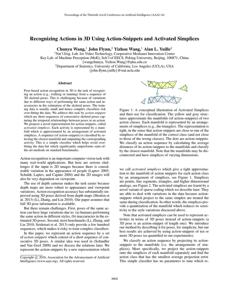
Figure 1: A conceptual illustration of Activated Simplices
and their use for classification. The yellow and gray structures approximate the manifolds (of action-snippets) of two
action classes. Each manifold is represented by an arrangements of simplices (e.g., the triangles). The representation is
tight, in the sense that action-snippets are close to one of the
simplices of the manifold of the correct class (and not close
to those of the wrong classes). The dots are action-snippets.
We classify an action sequence by calculating the average
distances of its action-snippets to the manifolds and classify
by the closest manifold. Note that the manifolds may be disconnected and have simplices of varying dimensions.
Action recognition is an important computer vision task with
many real-world applications. But here are serious challenges if the input is 2D images because there is considerable variation in the appearance of people (Laptev 2005;
Schuldt, Laptev, and Caputo 2004) and the 2D images will
also be very dependent on viewpoint.
The use of depth cameras makes the task easier because
depth maps are more robust to appearance and viewpoint
variations. Action recognition accuracy has substantially improved using 3D poses derived from depth maps (Shotton et
al. 2013) (Li, Zhang, and Liu 2010). Our paper assumes that
full 3D pose information is available.
But there remain challenges. First, poses of the same action can have large variations due to: (a) humans performing
the same action in different styles, (b) inaccuracies in the estimated 3D poses. Second, most benchmarks (Li, Zhang, and
Liu 2010; Seidenari et al. 2013) only provide a few hundred
sequences, which makes it risky to train complex classifiers.
In this paper, we represent an action sequence by a set
of action-snippets which consist of a short sequence of consecutive 3D poses. A similar idea was used in (Schindler
and Van Gool 2008) and we discuss the relations later. We
represent the action-snippets by a new representation which
we call activated simplices which give a tight approximation to the manifold of action snippets for each action class
by an arrangement of simplices, see Figure 1. Simplices
are points, line segments, triangles, and higher dimensional
analogs, see Figure 2. The activated simplices are learnt by a
novel variant of sparse coding which we describe later. They
are able to deal with variations in the data because actionsnippets which project to the same simplex are treated the
same during classification. In other words, the simplices provide a quantization of the manifold which reduces its sensitivity to the style variations discussed above.
Note that activated simplices can be used to represent activities in terms of 3D poses instead of action-snippets (a
3D pose is an action-snippet of length one). We introduce
our method by describing it for poses, for simplicity, but our
best results are achieved by using action-snippets of ten or
more 3D poses (as quantified in our experiments).
We classify an action sequence by projecting its actionsnippets to the manifolds (i.e. the arrangements of simplices). More specifically, we project the action-snippets
onto the simplices of each manifold separately and find the
action class that has the smallest average projection error.
This simple classifier has no parameters to tune which re-
c 2016, Association for the Advancement of Artificial
Copyright Intelligence (www.aaai.org). All rights reserved.
3604
x4
x3
Mixture-of-Structures Representations
x2
x1
Activated simplices represents a data manifold in terms of
an arrangement of simplices. This can be thought of as a
mixture-of-structures representation similar to k-means (i.e.
the centroids are analogous to the simplices). Activated simplices is a novel variant of sparse coding which enables
tight representations of data manifolds. It relates to methods which enforce group sparsity, but differs by learning
structure automatically instead of manually imposing group
structure (Bengio et al. 2009) or learning it by other techniques (Wang et al. 2011). We now describe related mixtureof-structures representations.
k-means partitions data into k Voronoi regions where each
region is represented by its mean. k-means is not a natural way to represent manifolds (see later for a comparison
to activated simplices). k-flats (Canas, Poggio, and Rosasco
2012) extends k-means by using a vocabulary of hyperplanes. The number of hyperplanes and their dimensions are
parameters of the model. k-flats has limited ability to model
curved manifolds because this requires many hyperplanes
for accurate reconstruction. Sparse subspace clustering(Elhamifar and Vidal 2013) groups data into hyperplanes by
analysing its self expression. The goal of Atlas (Pitelis, Russell, and Agapito 2013) is to fit the data by estimating local
hyperplane charts. Archetypal Analysis (Cutler and Breiman
1994) learns a global convex model for the data which can
cause problems if the data is not a convex set. Activated simplices is a novel mixture-of-structures representation which
has advantages over these standard models for the data in
this application (e.g., tightness of representation, ability to
deal with disconnected manifolds with varying dimensions,
and insensitivity to style variations)
x3
x1
x1
x2
x1
x2
Figure 2: Simplices of dimension 0,1,2 and 3. A 3-simplex
(far right) is a solid tetrahedron. Points within the tetrahedron are convex combinations
of the 4 vertices α1 x1 +
· · · α4 x4 , where αi ≥ 0 and αi = 1.
duces the risk of over-fitting when training data is small.
There are two main contributions in this work. First, we
propose a novel representation for 3D poses and actionsnippets which we call activated simplices (and which can
be applied to other forms of data). It approximates an action manifold in terms of an arrangement of simplices. This
gives a tight representation enabling us to classify sequences
based on the closest action manifold. Activated simplices
is a variant of sparse coding which is able to approximate
manifolds and which also relates to the mixture-of-structures
representation(e.g., k-means). Second, we propose a new
variant of action-snippets, which when coupled with activated simplices, yields a simple classifier which outperforms
state-of-the-art methods by a large margin.
Related Work
We briefly review related work on action recognition and
alternative representations to activated simplices.
3D Human Poses Based Action Recognition
There are three main approaches for action recognition
from depth data. One approach, e.g. (Oreifej and Liu 2013;
Wang et al. 2012a; Li, Zhang, and Liu 2010), extract features from dense depth maps and perform action classification. These methods give good results except in situations
where the background is complex (e.g., it would be hard to
segment the human from the background). We compare to
these methods in the experiments.
A second approach represents actions by 3D joint locations. Leading methods include: (i) computing spatial histograms of 3D joint locations and extracting discriminative
features by linear discriminant analysis (Xia, Chen, and Aggarwal 2012), (ii) computing pairwise joint position features
and using data mining to select the joints relevant to class labels (Wang et al. 2012b), and (iii) representing poses using a
set of dictionaries which are learned by group sparsity (Luo,
Wang, and Qi 2014). There are also some work (Rubinstein
and Elad 2014; Gu et al. 2014) learning discriminative dictionaries for classification tasks.
A third line of works groups body joints into body parts
by proposing a spatial-temporal-part model to capture the
differentiable configurations of body parts for classification
(Wang, Wang, and Yuille 2013). A similar idea of learning mid-level action representations was explored in (Wang
et al. 2015). Another leading method (Vemulapalli, Arrate,
and Chellappa 2014) models the geometric relations between body parts using rotations and translations. Actions
are treated as curves in Lie groups and classified by SVM.
Action-Snippets
The input to the action recognition task is a sequence of 3D
poses {y (1) , · · · , y (n) } where a pose y ∈ R3p is a vector
of p body joint locations. Some actions, e.g., standing up
and sitting down, are difficult to distinguish between by only
inspecting static poses. These two actions have similar poses
and it is their temporal order that make them different.
We incorporate the temporal order by combining consecutive poses together to form an action-snippet ŷ (Schindler
and Van Gool 2008) (ten poses give the best results, see
later). Then we represent an action by a sequence of actionsnippets: A = {ŷ (1) , · · · , ŷ (n−9) } where each ŷ (i) =
[y (i) · · · y (i+9) ]. Note that, unlike (Schindler and Van Gool
2008), our action-snippets overlap so the first action-snippet
starts at pose one, the second at pose two, and so on. This is
important if the pose sequences are not synchronized.
We learn a manifold for each action class, using activated
simplices as described in the next section. We classify an action sequence by first projecting all its action-snippets onto
each action manifold, as illustrated in Figure 1, and then calculating the projection error which we call the representation error. We select the action class which has smallest representation error when averaged over all the action-snippets
in the action sequence.
3605
essential to our approach.
First consider the inference problem of projecting y to the
closest point on the convex hull CX assuming that the bases
X are known (we discuss learning the bases later). This projection is done by minimizing the representation error:
y −
m
α i x i 2 ,
s.t.
i=1
m
αi = 1,
αi ≥ 0
(1)
i=1
Recall that the data y has norm y2 = 1 and lies on a sphere
which is outside the convex hull. Hence to minimize the representation error, each pose y must project to the boundary
(rather than to the interior) of the convex hull and hence to
one of the boundary simplices Δa ∈ F∂ . Hence identifying
which simplex the pose y projects to can simply be solved by
first solving the problem (1) and then identifying the boundary simplex which contains the activated bases (i.e. those
bases having non-zero α’s). This specifies the inference algorithm which determines how to identify a set of simplices
given training poses, if the bases X are known.
From another perspective, given a set of learned activated simplices F = {Δ1 , · · · , Δ|F | }, the model represents a pose y by its closest simplex Δa(y) : Δa(y) =
arg minΔa ∈F∂ Dist(Δa , y) where Dist(Δa , y) is the representation error of using simplex Δa to represent y.
The representation error is computed as Dist(Δa , y) =
ka
αi xai 2 with the non-negative and sum to
minα y − i=1
one constraints on α.
We now address the task of learning the bases and hence
the activated simplices from a set of training data {yμ : μ =
1, ..., N }. To learn the activated simplices we estimate the
bases X, which determines the convex hull CX , its boundary
∂CX , and then estimate which of the boundary simplices
are activated. The bases X are estimated by minimizing the
representation error of the training data:
Figure 3: The top and bottom rows show activated simplices
in 2D and 3D respectively. Data and bases (black points)
are on the unit sphere. The convex hull of the bases (red
and yellow) are inside the unit sphere. Data points (e.g., the
blue point) don not activate internal simplices (in blue) because the closest points in the convex hull lie on the facets, or
boundary simplices, (red segments and the yellow triangles)
of the convex hull. The activated simplices are the boundary
simplices which have data projected onto them.
The Activated Simplices
Activated simplices represent data by an arrangement of
simplices. It requires that the data has unit norm, which is a
reasonable requirement if the data is a 3D pose or an actionsnippet. The algorithm learns a set of unit basis vectors so
that the data is represented by simplices on the boundary of
the convex hull of the basis vectors.
The Activated Simplices representation is built on a set
of basis vectors X = {x1 , · · · , xm } which have norm one
(e.g., xi 2 = 1). The convex hull of the basis vectors
m X is
denoted by CX and contains all points of
form
i=1 αi xi
m
where αi ≥ 0 for all i = 1, · · · , m and i=1 αi = 1. The
boundary of the convex hull is ∂CX and it consists of a set of
boundary simplices F∂ . Each boundary simplex Δa ∈ F∂
has a set of basis vectors {xai : i = 1, · · · , ka }, where ka
is the number of basis vectors and ka − 1 is its dimension.
ka
αi xai , with αi ≥ 0 for
It consists of the set of points i=1
ka
all i = 1, · · · , ka and i=1 αi = 1. Boundary simplices of
the convex hull ∂CX have varying dimensions and can share
bases. This is illustrated in Figure 3 where the simplices are
either 1-simplices (lines) or 2-simplices (triangles).
The activated simplices F are a subset of the boundary
simplices, F ⊂ F∂ , which have a sufficient amount of data
projected onto them. Note that most subsets of basis vectors do not generate boundary simplices (a typical simplex
lies mostly within the convex hull CX ), see Figure 3. Indeed if there are m basis vectors in d dimensions then the
ratio of the number of boundary simplices to the total number of simplices is less than m−d/2 (Ziegler 2012). Hence
the number of activated simplices is typically much smaller
than the total number of simplices which puts restrictions on
the number of co-activation patterns of bases that can occur.
We apply activated simplices either to the poses y or to the
action-snippets ŷ. For simplicity we will only describe activated simplices for pose data (i.e. for action-snippets replace
y by ŷ). We normalize each pose so that it lies on the unit
sphere y2 = 1. This normalization ensures that the convex hull CX of the bases lies within the unit sphere which is
N
s.t.
μ=1
m
yμ −
m
αiμ xi 2
i=1
αiμ = 1,
αiμ ≥ 0,
(2)
for all i and μ
i=1
xi 2 ≤ 1,
for all i,
yμ 2 = 1,
for all μ
Note that we impose the constraint xi 2 ≤ 1 but the resulting bases are guaranteed to obey xi 2 = 1 (except for some
degenerate cases, which are easy to deal with). The bases
X directly determine the convex hull CX and its boundary
∂CX . The activated simplices are the boundary simplices
which correspond to a sufficient number of training data.
Solving the problem in equation (2) is equivalent to determining the bases X by minimizing the projection error
of the training data onto the boundary of the convex hull:
N
μ=1 minΔa ∈F∂ Dist(Δa , yμ ). At first sight, this second
formulation seems much harder because it is highly nonlinear in X (the boundary simplices F∂ are complex functions of the x s) and involves a correspondence problem
to determine the matching between the poses {yμ } and the
boundary simplices Δa ∈ F∂ . But, as discussed above, the
3606
c)
e)
0.13
0.12
g)
Activated Simplices
K−means
Sparse Coding
reconstruction error
0.11
0.1
0.09
0.08
0.07
b)
d)
f)
Relation to Sparse Coding
Activated simplices is related to sparse coding. Both represent the data by a sparse linear combination of bases and the
criteria to learn the bases, see equation (2), are very similar.
But there are some critical differences. Activated simplices
learns a mixture-of-structure representation (specified by the
co-activation patterns of the bases) which approximates the
data manifold, gives a tighter representation of the data than
sparse coding, and has some invariance to style variations.
In the standard formulation of sparse coding (Tibshirani
1996), (Osborne, Presnell, and Turlach 2000) data Y are represented by bases X through the 1 penalized optimization:
X,α
200
300
400
Number of bases
500
100
200
300
400
Number of bases
500
But this formulation can be modified to introduce positivity constraints (Huggins 2005) by making a negative copy
(−xi ) of each basis vector xi and representing αi xi by
max(αi , 0)xi + max(−αi , 0)(−xi ).
With this modification, we can think of sparse coding as
projecting the data onto the convex hull of the extended basis
vectors (X, −X). But, unlike activated simplices, the radius
of the convex hull αμ 1 varies depending on the datapoint
y and on the penalty λ. In other words, different datapoints
project to the convex hull of different scales.
Sparse coding and its variants, e.g., (Kyrillidis, Becker,
and Cevher 2012), differ from activated simplices in several respects. First, we normalize the data to lie on a unit
sphere. This seemingly trivial modification ensures that the
data is projected onto the boundary of the convex hull of the
bases and never into the interior. Second, the boundary of the
convex hull consists of a set of simplices which determines
the co-activation patterns of the bases and yields a mixtureof-structure representation. Hence activated simplices assign
each datapoint to one of |F∂ | labels. By contrast, sparse coding and its variants allow all combinations of basis vectors
to be used provided their sum α1 is small. Thirdly, sparse
coding yields a much less tight “prior” than activated simplices because there are many points Xα with small values
of α1 which do not correspond to real datapoints y (e.g.
poses violating the bending angle constraints). This is because there are many configurations with small α1 which
lie inside the convex hull CX while the data is close of the
boundary ∂CX (because it is normalized).
Figure 4 illustrates the difference between activated simplices and sparse coding. The data is the position of the hand
as the elbow joint is flexed (a). The manifold of valid poses
is an arc (b) of about 135 degrees. Panels (c,d) respectively
show the basis functions learnt by activated simplices and
sparse coding (three bases together with their negative counterparts). Activated simplices represents the data by an arrangement of two simplices on the boundary, see panel (e),
while sparse coding represents the data by the convex hull
of the bases in panel (f) paying a penalty α1 which encourages the data to lie near the center. Hence sparse coding
represents (i.e. pays a small α1 penalty for) data which
violates the constraint that arms cannot bend more than 135
degrees (h). By contrast, activated simplices can only represent data that are on the segments (e), which is a tighter
approximation of the manifold (i.e. the black curve (b)).
problem can be converted to an equivalent but easier problem which consists of two sub-problems: (i) learn the bases
X, and (ii) identify the boundary simplices that are activated
by the training poses which is a trivial task by inspecting the
non-zeros basis coefficients for each training pose.
In implementation, we initialize the basis vectors using
k-means initialized by k++ (Arthur and Vassilvitskii 2007).
The number of basis vectors is a parameter of the algorithm
(similar to the number of means in k-means). We minimize
(2) by an alternating algorithm adapted from sparse coding
(Mairal et al. 2009) which alternates between updating bases
X and coefficients α. When we fix alpha and update X, we
get the same optimization problem as Mairal 2009. When we
fix X and update alpha, we use an active-set method to optimize the QP problem with convex constraints. Then from
analysis of the activated coefficients we determine the activated simplices.
N
1 μ
y − Xαμ 2 + λαμ 1 .
N μ=1
0.1
0.09
Figure 5: Left: Representation errors on the H3.6M dataset
by activated simplices, sparse coding, and k-means. Right:
Representation errors when 1/3 of the data components
are missing. Activated simplices performs best on this case
showing that it gives a tight representation of the data.
h)
Figure 4: The difference between activated simplices and
sparse coding: a) The motion of the hand as the elbow is
flexed. b) The manifold of valid poses is an arc of the circle.
c) Three bases learned by Activated Simplices. d) The bases
and negative bases learned by sparse coding. e) The Activated Simplices. f) The convex hull of the bases and negative
bases. The activated simplices use two line segments while
sparse coding uses the convex hull, including the interior,
to approximate the manifold. So activated simplices gives a
tighter representation of the data than sparse coding. g) A
pose synthesized from the simplices. h) A pose synthesized
with small sparsity penalty overextends the elbow joint.
min
Activated Simplices
K−means
Sparse Coding
0.11
0.08
0.06
0.05
100
0.12
reconstruction error
a)
(3)
m μ
m
μ
μ
Here Xαμ =
i=1 αi xi , α 1 =
i=1 |αi |. In this
formulation there is no positivity constraint on the α s.
3607
Recognition accuracy
1
0.95
activated simplices
sparse coding
nearest−neighbor
Recognition accuracy
0.95
0.9
0.85
20
40
60
80
100 120
Number of bases per class
140
0.9
0.85
0.8
activated simplices
sparse coding
nearest−neighbor
0.75
0.7
2
4
6
8
Number of stacked poses
10
Figure 7: The influence of the number of bases (left panel)
and the number of poses in an action-snippet (right panel)
on action recognition accuracy.
Figure 6: This figure shows the reconstruction errors for
pose sequences of action classes 8 and 9 evaluated on all
the 20 classes. The x-axis is the class label and the y value
is the average reconstruction error. Each curve (including 20
points) denotes the average reconstruction errors of a test
sequence on the 20 action classes.
Experimental Results
We first evaluate how well activated simplices can represent
data by computing the distance between a data point and its
projection onto the nearest simplex. Then we present action
recognition results on three standard benchmark datasets
(Li, Zhang, and Liu 2010) (Seidenari et al. 2013) (Xia, Chen,
and Aggarwal 2012). We also provide diagnostic analysis.
Figure 8: Three sequences of 176 action-snippets of three
subjects are projected onto the activated simplices of the
“punch forward” class. Each color represents a simplex. The
snippets of different subjects are projected to similar simplices which suggests the model is robust to style variations.
Human Pose Reconstruction
We conduct experiments on a large human pose dataset
H3.6M (Ionescu et al. 2014). We use 11, 000 3D poses of 11
actions including “taking photo”, “smoking”, “purchases”
“discussion”, etc from the dataset to evaluate our method.
We split the 11, 000 poses into training and testing subsets
each containing 5, 500 poses of the 11 actions. We compare
with two baseline methods: k-means and sparse coding. For
k-means, we learn a dictionary consisting of all the cluster
centers and reconstruct a pose by the nearest element in the
dictionary. Similarly for sparse coding, we learn a dictionary
of bases by the method of sparse coding (Mairal et al. 2009)
and reconstruct a pose by the dictionary with 1 -norm regularization on the coefficients α.
Figure 5 (left) shows the results. K-means method has the
largest errors because the poses are coarsely quantized by
the nearest centers. By contrast, sparse coding and activated
simplices use combinations of the bases to represent the data
more accurately. We see that activated simplices achieves
almost the same performance as sparse coding, even though
activated simplices restricts the co-activations of the bases.
Next we investigate how tightly activated simplices represents poses if we only have partial information. As discussed earlier, sparse coding makes no restrictions on the
co-activations of the bases and hence can represent data that
are not from the manifold; see Figure 4. This is a limitation
for regularization tasks such as estimating the 3D pose with
partial information. To illustrate this, we compare the performance of k-means, sparse coding, and activated simplices
for reconstructing partially visible poses. In this experiment,
we recover the depth component of the pose (i.e. we remove
the depth information from the testing data). This is done
by setting the z components of the poses to be zero as well
as the corresponding components of the basis vectors. Lifting the data back onto the activated simplices recovers the z
components. Figure 5 (right) shows the results. We can see
that activated simplices performs better than sparse coding
and k-means. hence justifying that it provides a tighter representation of the data manifold. This is an important property
for classification tasks which we will discuss later.
Finally, we investigate the sensitivity of activated simplices to style variations. Figure 8 shows that action-snippets
of the same action, performed by different people, are often
projected onto the same simplices.
Action Recognition
Now we evaluate our approach on the action recognition task
on three benchmark datasets: the MSR-Action3D dataset,
the Florence dataset and the UTKinect dataset.
The MSR-Action3D Dataset This dataset (Li, Zhang, and
Liu 2010) provides 557 human pose sequences of ten subjects performing 20 actions which are recorded with a depth
sensor. Many works choose five subjects for training and the
remaining subjects for testing, e.g. in (Li, Zhang, and Liu
2010), and report the result based on a single split. But it was
shown in (Padilla-López, Chaaraoui, and Flórez-Revuelta
2014) that the choice of data splits (i.e. which five subjects
were selected for training) has a large influence on the results. To make the results more comparable we experiment
with all 252 possible splits and report the average accuracy.
We set the number of bases for each class to be 40 (by
cross-validation). We obtain about 15 activated simplices,
whose dimensions are five on average, for each class, activated simplices achieves recognition accuracy of 91.40%.
Figure 6 show the errors of projecting a pose sequence
onto all the action classes (the lowest error occurs when we
project onto the correct class). We can also determine which
classes are most easy to confuse. For example, from Figure
6 we see that the class 8 and class 9 are difficult to distinguish between. The classes correspond to the “draw tick”
3608
Table 1: Average action recognition accuracy of all 252 5-5
splits on MSR-Action3D.
Methods
HON4D (Oreifej and Liu 2013)
Rahmani et al. (Rahmani et al. 2014)
Tran et al. (Tran and Ly 2013)
Our Approach
Table 2: Action recognition accuracy on the Florence dataset
using leave-one-actor-out setting.
Accuracy (%)
82.15
82.70
84.54
91.40
Methods
Seidenari et al.2013
Vemulapalli et al.2014
Devanne et al.2015
Our Approach
Accuracy (%)
82.15
90.88
87.04
94.25
Table 3: Action recognition accuracy using leave-onesequence-out setting on the UTKinect dataset.
and “draw circle” actions, which are indeed similar.
Comparison with Three Baselines: The first baseline
uses nearest neighbors to classify the action-snippets. This
has recognition accuracy of 85.16% which is lower than activated simplices (presumably because our method can handle performing style variations well; see Figure 8).
The second baseline is the k-means method. Given a sequence of action-snippets, we compute their distances to
(nearest center of) each class and classify by the nearest
class. The performance is about 79.30%. This is lower than
our method which is mainly because of the coarse quantization.
The third baseline is sparse coding (and a variant). We
learn independent bases for the 20 classes. The number of
bases is the same as for activated simplices. We project the
action-snippets onto the bases of 20 classes. The class that
achieves the least average error is the prediction. The accuracy for sparse coding is 86.30% which is lower than our
method (presumably because sparse coding is less tight).
The accuracy for a variant of sparse coding with nonnegative and sum to one constraint on coefficients, is 86.94%
which is not significantly better than standard sparse coding. This is mainly because –Enforcing the constraints gives
a tighter representation than standard sparse coding. But, it
doesn’t identify, and so does not exploit, co-activation patterns (unlike our method).
We also evaluated the influence of the two main parameters in the model, i.e. the number of bases and the number
of poses in each action snippet. We report the average performance based on ten random splits. Figure 7 shows the results. Activated simplices achieves better performance as the
number of bases increases but the increase is small when the
number exceeds 50. Sparse coding obtains best performance
when the number is 20. The performance goes down quickly
as we allow more bases, presumably because the sparse coding becomes less tight as the number of bases becomes big.
The nearest neighbor method uses no bases hence the performance is constant. From the right sub-figure, we can see
that increasing the number of poses in the action-snippets
consistently improves the performance.
Comparison with the State-of-the-art: Table 1 compares activated simplices with state-of-the-art methods using
the protocol of “average over all splits”. We can see that our
method outperforms three state-of-the-art methods. In addition, our method is arguably the simplest.
Since some recent methods only provide results for a single split, we also provide these results. However, note that
they are not directly comparable as they may choose different five subjects for training. For our method, the split using
Methods
(Devanne et al. 2015)
(Xia, Chen, and Aggarwal 2012)
Our Approach
Accuracy (%)
91.50
90.92
96.48
training subjects 1,3,5,7,9 achieves accuracy of 95.03% and
our highest accuracy is 99.25%. (Luo, Wang, and Qi 2014)
achieve recognition accuracy of 96.70% and (Vemulapalli,
Arrate, and Chellappa 2014) achieve 89.48%.
The Florence Dataset This dataset (Seidenari et al. 2013)
includes nine activities including wave, drink from a bottle,
etc. The background is very cluttered in this dataset. Ten
subjects were asked to perform the above actions. Following
the dataset recommendation, we use a leave-one-actor-out
protocol: we train the classifier using all the sequences from
nine out of ten actors and test on the remaining one. We
repeat this procedure for all actors and compute the average
classification accuracy values of the ten actors.
We set the number of bases for each class to be 50 (450
in total) by cross-validation. Table 2 compares our method
with the state-of-art methods on this dataset. Our approach
achieves the highest recognition accuracy.
The UTKinect Dataset This dataset (Xia, Chen, and Aggarwal 2012) was captured using a single stationary Kinect.
There are ten action types including walk, sit down, stand
up, etc. Each action is performed by ten subjects.
We learn 40 bases and about 20 activated simplices for
each action class. The dimension of the simplices is five on
average. We use the standard “leave-one-sequence-out” protocol where one sequence is used for testing and the remaining are used for training. We repeat this process for all sequences and report the average accuracy. Table 3 shows the
results. Our approach achieves the best performance.
Learning and Inference Efficiency Learning the bases
and the activated simplices for the above three datasets takes
several seconds. Inferring the class labels (i.e. projecting
poses onto the activated simplices) can be done in real time.
Conclusion
This paper has two main contributions. The first is activated
simplices which is a novel variant of sparse coding which
yields a tight mixture-of-structure representation. The second contribution is the use of action-snippets. We evaluated
3609
our approach on three benchmark datasets and showed that
it outperforms the state-of-the-arts.
Acknowledgements: We thank Xianjie Chen for helping improve the writing, and for support from the following research grants 973-2015CB351800, the Okawa Foundation Research Grant, NSFC-61272027, NSFC-61231010,
NSFC-61527804, NSFC-61421062, NSFC-61210005, ONR
grant N00014-15-1-2356 and ARO 62250-CS. We also
thank NVIDIA Corporation for donating the GPUs.
compare human action recognition methods using the msr
action3d dataset. arXiv preprint arXiv:1407.7390.
Pitelis, N.; Russell, C.; and Agapito, L. 2013. Learning a
Manifold as an Atlas. In CVPR, 1642–1649.
Rahmani, H.; Mahmood, A.; Huynh, D. Q.; and Mian, A.
2014. Real time action recognition using histograms of depth
gradients and random decision forests. In WACV, 626–633.
IEEE.
Rubinstein, R., and Elad, M. 2014. Dictionary learning
for analysis-synthesis thresholding. Signal Processing, IEEE
Transactions on 62(22):5962–5972.
Schindler, K., and Van Gool, L. 2008. Action snippets:
How many frames does human action recognition require?
In CVPR, 1–8. IEEE.
Schuldt, C.; Laptev, I.; and Caputo, B. 2004. Recognizing
human actions: a local svm approach. In ICPR, volume 3,
32–36. IEEE.
Seidenari, L.; Varano, V.; Berretti, S.; Del Bimbo, A.; and
Pala, P. 2013. Recognizing actions from depth cameras as
weakly aligned multi-part bag-of-poses. In CVPRW, 479–
485. IEEE.
Shotton, J.; Sharp, T.; Kipman, A.; Fitzgibbon, A.; Finocchio, M.; Blake, A.; Cook, M.; and Moore, R. 2013. Realtime human pose recognition in parts from single depth images. Communications of the ACM 56(1):116–124.
Tibshirani, R. 1996. Regression shrinkage and selection via
the lasso. Journal of the Royal Statistical Society. Series B.
Methodological 267–288.
Tran, Q. D., and Ly, N. Q. 2013. Sparse spatio-temporal
representation of joint shape-motion cues for human action
recognition in depth sequences. In Computing and Communication Technologies, Research, Innovation, and Vision for
the Future (RIVF), 2013 IEEE RIVF International Conference on, 253–258. IEEE.
Vemulapalli, R.; Arrate, F.; and Chellappa, R. 2014. Human
action recognition by representing 3d skeletons as points in
a lie group. In CVPR, IEEE Conference on, 588–595. IEEE.
Wang, F.; Lee, N.; Sun, J.; Hu, J.; and Ebadollahi, S. 2011.
Automatic group sparse coding. In AAAI.
Wang, J.; Liu, Z.; Chorowski, J.; Chen, Z.; and Wu, Y. 2012a.
Robust 3d action recognition with random occupancy patterns. In ECCV. Springer. 872–885.
Wang, J.; Liu, Z.; Wu, Y.; and Yuan, J. 2012b. Mining actionlet ensemble for action recognition with depth cameras.
In CVPR, IEEE Conference on, 1290–1297. IEEE.
Wang, Y.; Wang, B.; Yu, Y.; Dai, Q.; and Tu, Z. 2015.
Action-gons: Action recognition with a discriminative dictionary of structured elements with varying granularity. In
ACCV. Springer. 259–274.
Wang, C.; Wang, Y.; and Yuille, A. L. 2013. An Approach
to Pose-Based Action Recognition. In CVPR, 915–922.
Xia, L.; Chen, C.-C.; and Aggarwal, J. 2012. View invariant
human action recognition using histograms of 3d joints. In
CVPR, 20–27. IEEE.
Ziegler, G. M. 2012. Lectures on Polytopes. Springer Science
& Business Media.
References
Arthur, D., and Vassilvitskii, S. 2007. k-means++: The advantages of careful seeding. Proceedings of the eighteenth
annual ACM- . . . .
Bengio, S.; Pereira, F.; Singer, Y.; and Strelow, D. 2009.
Group sparse coding. In NIPS, 82–89.
Canas, G. D.; Poggio, T. A.; and Rosasco, L. 2012. Learning
Manifolds with K-Means and K-Flats. NIPS.
Cutler, A., and Breiman, L. 1994. Archetypal analysis. Technometrics 36(4):338–347.
Devanne, M.; Wannous, H.; Berretti, S.; Pala, P.; Daoudi, M.;
and Del Bimbo, A. 2015. 3-d human action recognition by
shape analysis of motion trajectories on riemannian manifold. Cybernetics, IEEE Transactions on 45(7):1340–1352.
Elhamifar, E., and Vidal, R. 2013. Sparse subspace clustering: Algorithm, theory, and applications. PAMI 35(11):2765–
2781.
Gu, S.; Zhang, L.; Zuo, W.; and Feng, X. 2014. Projective
dictionary pair learning for pattern classification. In NIPS,
793–801.
Huggins, P. S. 2005. Sparse Coding via Geometry. Ph.D.
Dissertation, Yale University.
Ionescu, C.; Papava, D.; Olaru, V.; and Sminchisescu, C.
2014. Human3.6m: Large scale datasets and predictive methods for 3d human sensing in natural environments. PAMI
36(7):1325–1339.
Kyrillidis, A. T.; Becker, S.; and Cevher, V. 2012. Sparse
projections onto the simplex. CoRR abs/1206.1529.
Laptev, I. 2005. On space-time interest points. IJCV.
Li, W.; Zhang, Z.; and Liu, Z. 2010. Action recognition
based on a bag of 3d points. In (CVPRW), 2010 IEEE Conference on, 9–14. IEEE.
Luo, J.; Wang, W.; and Qi, H. 2014. Group sparsity and geometry constrained dictionary learning for action recognition
from depth maps. In CVPR. IEEE.
Mairal, J.; Bach, F.; Ponce, J.; and Sapiro, G. 2009. Online
dictionary learning for sparse coding. ICML 689–696.
Oreifej, O., and Liu, Z. 2013. Hon4d: Histogram of oriented
4d normals for activity recognition from depth sequences. In
CVPR, 716–723. IEEE.
Osborne, M. R.; Presnell, B.; and Turlach, B. A. 2000. On the
LASSO and its dual. Journal of Computational and Graphical Statistics 9(2):319–337.
Padilla-López, J. R.; Chaaraoui, A. A.; and Flórez-Revuelta,
F. 2014. A discussion on the validation tests employed to
3610