Proceedings of the Thirtieth AAAI Conference on Artificial Intelligence (AAAI-16)
Efficient Nonparametric Subgraph Detection Using Tree Shaped Priors
Nannan Wu∗
∗
Feng Chen†
Jianxin Li∗ § Baojian Zhou†
Naren Ramakrishnan‡
Dept. of Computer Science & Engineering, Beihang University, Beijing 100191, China
†
Dept. of Informatics, University at Albany, SUNY, Albany, NY 12203
‡
Dept. of Computer Science, Virginia Tech, Arlington, VA 22203
{wunannan, lijx}@act.buaa.edu.cn {fchen5, bzhou6}@albany.edu naren@cs.vt.edu
Abstract
Non-parametric graph scan (NPGS) statistics are used
to detect anomalous connected subgraphs on graphs,
and have a wide variety of applications, such as disease outbreak detection, road traffic congestion detection, and event detection in social media. In contrast to
traditional parametric scan statistics (e.g., the Kulldorff
statistic), NPGS statistics are free of distributional assumptions and can be applied to heterogeneous graph
data. In this paper, we make a number of contributions
to the computational study of NPGS statistics. First,
we present a novel reformulation of the problem as a
sequence of Budget Price-Collecting Steiner Tree (BPCST) sub-problems. Second, we show that this reformulated problem is NP-hard for a large class of nonparametric statistic functions. Third, we further develop
efficient exact and approximate algorithms for a special
category of graphs in which the anomalous subgraphs
can be reformulated in a fixed tree topology. Finally,
using extensive experiments we demonstrate the performance of our proposed algorithms in two real-world
application domains (water pollution detection in water sensor networks and spatial event detection in social media networks) and contrast against state-of-theart connected subgraph detection methods.
1
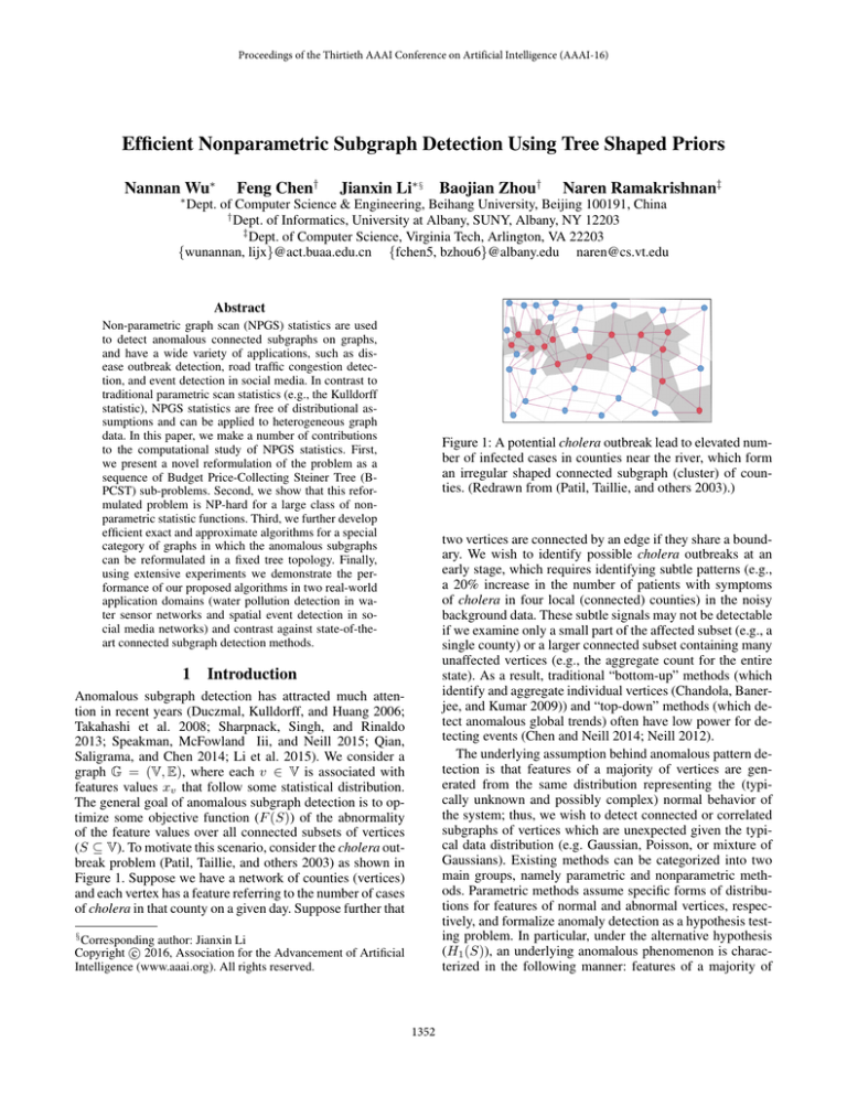
Figure 1: A potential cholera outbreak lead to elevated number of infected cases in counties near the river, which form
an irregular shaped connected subgraph (cluster) of counties. (Redrawn from (Patil, Taillie, and others 2003).)
two vertices are connected by an edge if they share a boundary. We wish to identify possible cholera outbreaks at an
early stage, which requires identifying subtle patterns (e.g.,
a 20% increase in the number of patients with symptoms
of cholera in four local (connected) counties) in the noisy
background data. These subtle signals may not be detectable
if we examine only a small part of the affected subset (e.g., a
single county) or a larger connected subset containing many
unaffected vertices (e.g., the aggregate count for the entire
state). As a result, traditional “bottom-up” methods (which
identify and aggregate individual vertices (Chandola, Banerjee, and Kumar 2009)) and “top-down” methods (which detect anomalous global trends) often have low power for detecting events (Chen and Neill 2014; Neill 2012).
The underlying assumption behind anomalous pattern detection is that features of a majority of vertices are generated from the same distribution representing the (typically unknown and possibly complex) normal behavior of
the system; thus, we wish to detect connected or correlated
subgraphs of vertices which are unexpected given the typical data distribution (e.g. Gaussian, Poisson, or mixture of
Gaussians). Existing methods can be categorized into two
main groups, namely parametric and nonparametric methods. Parametric methods assume specific forms of distributions for features of normal and abnormal vertices, respectively, and formalize anomaly detection as a hypothesis testing problem. In particular, under the alternative hypothesis
(H1 (S)), an underlying anomalous phenomenon is characterized in the following manner: features of a majority of
Introduction
Anomalous subgraph detection has attracted much attention in recent years (Duczmal, Kulldorff, and Huang 2006;
Takahashi et al. 2008; Sharpnack, Singh, and Rinaldo
2013; Speakman, McFowland Iii, and Neill 2015; Qian,
Saligrama, and Chen 2014; Li et al. 2015). We consider a
graph G = (V, E), where each v ∈ V is associated with
features values xv that follow some statistical distribution.
The general goal of anomalous subgraph detection is to optimize some objective function (F (S)) of the abnormality
of the feature values over all connected subsets of vertices
(S ⊆ V). To motivate this scenario, consider the cholera outbreak problem (Patil, Taillie, and others 2003) as shown in
Figure 1. Suppose we have a network of counties (vertices)
and each vertex has a feature referring to the number of cases
of cholera in that county on a given day. Suppose further that
§
Corresponding author: Jianxin Li
c 2016, Association for the Advancement of Artificial
Copyright Intelligence (www.aaai.org). All rights reserved.
1352
the vertices are generated from the same background distribution, and features of perhaps a small connected subset
S ⊆ V of vertices are generated from a different distribution. The goal is to maximize an appropriate set function
1 (S))
(F (S)), typically the likelihood ratio F (S) = Pr(Data|H
Pr(Data|H0 ) ,
over all possible connected subsets S (with H0 being the
null hypothesis). Depending on the specific forms of distributions assumed, a number of methods have been proposed,
including an expectation-based Poisson statistic (Neill et al.
2005), the Kulldorff statistic (Kulldorff 1997), the elevated
mean scan statistic (Qian, Saligrama, and Chen 2014), and
various others.
Nonparametric methods do not associate specific forms
of distributions with normal and abnormal vertices. Instead,
they first estimate a p-value for each vertex based on empirical calibration by comparing the current features of this vertex with its features in the historical data for the vertex (Chen
and Neill 2014; McFowland, Speakman, and Neill 2013).
This approach then maximizes a score function F (S) of pvalues in S, typically nonparametric scan statistic measuring the significance of the collection of p-values in S, over
all possible connected subsets. A number of NPGS statistic functions have been proposed in recent years, including the Berk-Jones (BJ) statistic (Berk and Jones 1979), the
Higher Criticism (HC) statistic (Donoho and Jin 2004), the
Tippet’s statistic, rank truncated statistic, and various others. Note that these nonparametric statistic functions were
originally proposed to combine p-values from a set of hypothesis tests in the area of statistical meta analysis. Recent studies show that these functions can be satisfactorily
used with NPGS for detecting anomalous subgraphs (McFowland, Speakman, and Neill 2013; Chen and Neill 2014;
Bogdanov, Mongiovı̀, and Singh 2011). The main contributions of our study are summarized as follows:
Figure 2: The BJ statistic scores of the three example subgraphs demonstrate that this score function increases with
Nα (S) and decreases with N (S) − Nα (S) and α. Yellowcolored vertices refer to the vertices whose p-values are less
than or equal to α.
of edges, and the mapping function p : V → [0, 1] defines
a single empirical p-value to each vertex v, which can be
calculated based on empirical calibration by comparing current features of v with its features in the historical data for
v (Chen and Neill 2014; McFowland, Speakman, and Neill
2013). The general form of the Non-Parametric Graph Scan
(NPGS) statistic (Chen and Neill 2014; McFowland, Speakman, and Neill 2013) is defined as:
F (S) = max Fα (S) = max φ(α, Nα (S), N (S)), (1)
α
• Hardness Analysis. We reformulate the NPGS problem
as a sequence of B-PCST sub-problems, and show that
this reformulated problem is NP-hard for a general category of nonparametric statistic functions. These functions
satisfy two intuitive properties on the cardinality of the
input subgraph S and the number of vertices in S that are
significant at a confidence level α.
• Exact and approximate algorithms for graphs with
tree shaped priors. We develop efficient algorithms to
the NPGS problem that are guaranteed to find an optimal
solution in worst-case time O(N 3 ) and an approximate
solution in worst-case time O(N 2 /) when the connected
subgraph can be reformulated in a fixed tree topology.
• Comprehensive experiments to validate the effectiveness and efficiency of the proposed techniques. We conduct extensive experiments on a water sensor dataset and a
Weibo dataset. The results demonstrate that our proposed
algorithms outperform existing representative techniques
in both performance and quality.
2
α
where S ⊆ V refers
to a connected set of vertices (subis the number of pgraph), Nα (S) = v∈S δ(p(v) ≤ α) values significant at level α, N (S) =
v∈S 1 is the total
number of p-values in S. The function δ(·) =
1 if its input is
True, otherwise δ(·) = 0. Denote N̄α (S) = v∈S δ(p(v) >
α), which means that N (S) = N̄α (S) + Nα (S). The significance level α can be optimized between 0 and some constant αmax (0.15 by default). We assume that the function
φ(α, Nα (S), N (S)) satisfies two intuitive properties:
(P1) φ is monotonically increasing w.r.t. Nα (S),
(P2) φ is monotonically decreasing w.r.t. N (S) − Nα (S).
These assumptions follow naturally because the score φ increases with the number of significant p-values and deceases
with the number of insignificant p-values at the level α. The
importance to consider a range of α in the function is discussed in (Chen and Neill 2014). The range of α refers to
the set of all possible p-values in G between 0 and α.
This paper presents efficient algorithms for the large class
of nonparametric scan statistics that satisfy the above two
properties, such as the Berk-Jones (BJ) statistic (Berk and
Jones 1979), the Higher Criticism (HC) statistic (Donoho
and Jin 2004), the Kolmogorov-Smirnov statistic, the
Davidov-Herman statistic, and the chi-bar squared statistic.
For illustration purpose, we consider the first two functions.
The BJ statistic is defined as:
Nα (S)
, α , (2)
ϕBJ (α, Nα (S), N (S)) = N (S) × KL
N (S)
where KL is the Kullback-Liebler divergence between the
observed and expected proportions of p-values less than α.
The HC statistic is defined as:
Nα (S) − N (S)α
ϕHC (α, Nα (S), N (S)) = .
(3)
N (S)α(1 − α)
Nonparametric Graph Scan Statistics
Given a graph G(V, E, p) where V = {v1 , ..., vN }, N refers
to the total number of vertices, E ⊆ V × V refers to the set
1353
Figure 3: (a) An illustration of our work to decompose NPGS problem into a sequence of K-budget subgraph detection problems. (b) With the number of normal vertices is equal to K, including v, we aim to find a solution including more abnormal
+
vertices. We consider assigning the value of πK
in vertex V as a multiple-choice knapsack problem from π + of children V1,...,h .
MCK refers to multiple choice knapsack.
Proof. This theorem can be proved by contradiction. Suppose (α̂, Ŝ) is not an optimal solution to the NPGS problem. It follows that there exists a different solution (α∗ , S ∗ ),
such that φ(α∗ , Nα∗ (S ∗ ), N (S ∗ )) > φ(α̂, Nα̂ (Ŝ), N (Ŝ)).
Let K̂ := N (Ŝ) − Nα̂ (Ŝ) and K ∗ := N (S ∗ ) − Nα∗ (S ∗ ).
We first observe that Nα∗ (VT K∗∗ ) = Nα∗ (S ∗ ); Otherα
wise, VT K∗∗ will be the optimal subset, instead of S ∗
α
due to (P1) and (P2). Similarly, it can be shown that
Nα̂ (VT K̂ ) = Nα̂ (Ŝ). As (α̂, Ŝ) is the optimal solution to
α̂
the reformulated problem (6), the inequality must be true:
φ(α∗ , Nα∗ (S ∗ ), N (S ∗ )) ≤ φ(α̂, Nα̂ (Ŝ), N (Ŝ)), a contradiction. Therefore, the initial assumption – (α̂, Ŝ) is not an
optimal solution to the NPGS problem – must be false.
Given a selected nonparametric scan statistic function
ϕ(α, Nα (S), N (S)), the detection of the most anomalous
connected subgraph from V can be formalized as the following optimization problem:
max φ(α, Nα (S), N (S)),
max
S⊆V:S is connected α≤αmax
(4)
which is equivalent to the problem:
max
max
α∈U(V,αmax ) S⊆V:S is connected
φ(α, Nα (S), N (S)),
(5)
where U(V, αmax ) refers to the union of {αmax } and the set
of distinct p-values less than αmax in V.
3
Methodology
This section presents a new reformulation of the NPGS
problem and develops efficient algorithms for a special category of graph data where the connectivity constraint of the
subgraph can be reformulated in a fixed tree topology.
3.1
Theorem 2 (Hardness). The reformulated problem (6) is
NP-hard for the large class of nonparametric scan statistics
that satisfy (P1) and (P2).
Proof. Each subproblem (7) is a binary-case B-PCST problem that is known to be NP-hard (Johnson, Minkoff, and
Phillips 2000). It can then be readily proved that the reformulated problem (6) is NP-hard.
Problem Reformulation
The hardness analysis of the NPGS problem is difficult as
it involves a nonlinear objective function, and can not be
reduced from known NP-hard problems that often involve
linear objective functions. The following theorem shows that
the NPGS problem can be reformulated a sequence of BPCST sub-problems, and the hardness of the reformulated
problem can be readily analyzed.
Theorem 1 (NPGS Reformulation). The NPGS problem
(5) is equivalent to the following problem:
(α̂, Ŝ) =
max
max
0 ,...,S N }
α∈U(V,αmax ) Sα ∈{Sα
α
3.2
φ(α, Nα (S), N (S))
(6)
where each SαK = VTαK , and TαK is the optimal subtree
of the budget node-weighted Prize-Collecting Steiner Tree
problem (B-PCST):
TαK = max
πα (v), s.t.
cα (v) ≤ K, (7)
T ∈T(G)
v∈VT
Approximations with tree shaped priors
Although the B-PCST sub-problem (7) can be approximated
with the factor of O(log N ) in polynomial time (Bateni, Hajiaghayi, and Liaghat 2013), both the Big-O approximation
factor and the polynomial time complexity of this approximation are not satisfactory for large graph analysis. To design more efficient solutions for the subproblem (7), we propose to reformulate the connectivity constraint of the subgraph S on a fixed topology. Particularly, we approximate
the graph G as a tree Tr originating at a given root vertex
r ∈ V, and the search of the best connected subgraph S for
the NPGS problem is approximated as the search of the best
sub-tree in Tr . There are several heuristics to find the tree for
the input graph: (1) breadth-first tree; (2) random spanning
tree; (3) steiner tree; and (4) geodesic shortest path tree. The
first three tree heuristics have been successfully applied to
discrepancy maximization on general graphs (Gionis, Mathioudakis, and Ukkonen 2015). The fourth tree heuristic has
v∈VT
where T(G) ≡ {T = (VT , ET )} denotes the set of sub-trees
of G, πα (v) = 1 and cα (v) = 0, if p(v) ≤ α; otherwise,
πα (v) = 0 and cα (v) = 1.
1354
• Clv : a set of tuples of the form (v , t). Hereby, v is a child
of v and t is an integer number that denotes the size of the
sub-tree to be collected in T (v ).
• C(v): the set of children of v in T (v).
The DP procedure is presented as follows:
Leaf vertex: We set initial values to attributes of leaf ver−v
= 0,
tices. For a leaf vertex v, if p(v) > α, set πl∈{0,1}
+v
v
= 0 and svl∈{0,1} = F alse, and if
πl∈{0,1} = 0, πl∈{0,1}
p(v) ≤ α, set π0+v = 1, π0v = 1 and sv0 = T rue.
Non-leaf vertex: Attributes nvl and πl−v are computed as:
been successfully applied to image segmentation and sensor
networks (Stühmer, Schröder, and Cremers 2013).
Breadth-First Tree (BFS-Tree): From random candidate
root vertices, it generates a breadth-first tree for each root.
Random Spanning Tree (Random-ST): We get a random
tree by assigning a weight (uniformly from [0, 1]) to each
edge, and computing the minimum weight spanning tree.
Steiner Tree (Steiner-T): Intuitively, a tree is good if abnormal vertices are interconnected with the least number of normal vertices. For each α ∈ U(V, αmax ), if we denote each
abnormal vertex as a terminal vertex, and each normal vertex as a steiner vertex, trees can be identified by generating
the steiner trees of the input graph.
Geodesic Shortest Path tree (Geodesic-SPT): For the
NPGS problem, we define the optimal cost of the connecting path p between a fixed vertex s and other x based on the
statistic: exp{− maxα φ(α, Nα (Sp ), N (Sp ))} (Stühmer,
Schröder, and Cremers 2013), where Sp are vertices in p.
The tree can be got through (Narvez, Siu, and Tzeng 2000).
3.3
nv
nvl = max{πlv1 , · · · , πlvh }, πl−v = πl l ,
vi
where {v1 , · · · , vh } refer to the h child vertices of the vertex v. As illustrated in Figure 3 (b), the computation of the
attribute πl+v can be reduced to a 0-1 multiple-choice knapsack (0-1 MCK) problem that has the approximation factor
(1+) and the running time O(Kh/) (Bansal and Venkaiah
). The problem is to select at most one πj+vi from each child
i = {1, · · · , h} such that the sum of profit is maximized
without summing budget j to exceed l − δ(p(v) > α). πl+v
can then be calculated as:
Dynamic algorithms for the problem (7)
When the input graph G is a tree T (r) with the root vertex
r, we can solve the problem (7) optimally, using dynamic
programming (DP). We first introduce a few notations:
πl+v = max δ(p(v) ≤ α) +
• T (v): a sub-tree of G with the root vertex v.
x
• πl−v : the value of the best l-budget sub-tree to the problem
(7) in T (v) that does not contain v.
• πlv : πlv = max{πl−v , πl+v }.
πj+vi · xi,j
(9)
(10)
We compute DP(K, Tv0 , v0 , α) using two-stages: 1) Calculate {πl−v , πl+v , πlv , svl , nvl , Clv }K
l=0 for v ∈ V; 2) From the
svK = T rue. Set SαK ←
root vertex v0 down, we find the first
Φ, compute f indchild(T , v, l) = (vi ,j)∈C v SαK ∪ {vi } ∪
l
f indchild(T , vi , j) and last return f indchild(T , svK , K).
The detailed information of the implementation can be
found from the online appendix (Wu et al. ).
Theorem 3. 1) Exact Solution: If each 0-1 MCK subproblem (9) is solved via dynamic programming (Pisinger
1994), Algorithm 1 is guaranteed to find the optimal solution
to the tree-priors-based NPGS problem in worst-case time
O(|U(V, αmax )| · N 3 ); 2) Approximate Solution: If each 01 MCK subproblem (9) is solved via the algorithm (Bansal
and Venkaiah ) that has the approximation factor (1 + ),
then Algorithm 1 is guaranteed to find an approximate solution to the tree-priors-based NPGS problem in worst-case
time O(|U(V, αmax )| · N 2 /).
• nvl : a vertex pointer that indicates to which child of v to
find the best l-budget sub-tree, if svl = F alse.
Algorithm 1: Tree-Shaped-Priors Subgraph Detection
Input: Graph G(V, E, p)
Result: The most anomalous subgraph S ∗
1 Set αmax = 0.15 and C = 5;
2 for c ∈ {1, · · · , C} do
3
Select seed v0 from {v|v ∈ V, p(v) ≤ αmax };
4
Approximate the graph G as a tree T (v0 );
5
for α ∈ U(V, αmax ) do
6
for K = 0, · · · , N (V) − Nα (V) do
7
SαK ← DP(K, Tv0 , v0 , α) in Section 3.3;
8
end
9
end
10
S c = arg max φ(α, Nα (SαK ), N (SαK ));
Proof. An 0-1 MCK subproblem will be solved for each vertex vi with the time O(K 2 hi ) for exact solutions via dyi
namic programming (Pisinger 1994) and the time O( Kh
)
for approximate solutions (Bansal and Venkaiah ), where hi
refers
to the number of child vertices of vi . As K → N and
vi ∈V hi + 1 = N , the times can be readily proved.
α∈U(V,αmax ),K
13
i=1 j=0
Clv = {(vi , j)|xi,j = 1}.
• svl : a boolean value that indicates if vertex v belongs to
the best l-budget sub-tree in T (v).
12
h K
h K
K
s.t. j=0 xi,j ≤ 1, i = {1, · · · , h}, i=1 j=0 j ·xi,j ≤
l − δ(p(v) > α), where x ∈ {0, 1}h×K . Set svl = F alse if
πl−v > πl+v , otherwise svl = T rue. Given the result x from
the problem (9), the set attribute Clv can be calculated as:
• πl+v : the value of the best l-budget sub-tree to the problem
(7) in T (v) that contains v.
11
(8)
end
Calculate c∗ = arg maxc φ(α, Nα (S c ), N (S c ));
∗
return S c
1355
Method
BFS-Tree (BJ)
Random-ST (BJ)
Steiner-T (BJ)
Geodesic-SPT (BJ)
EventTree
NPHGS (BJ)
LTSS (BJ)
Graph-Laplacian
Noise Ratio (0%)
0.94, 0.48 (0.64)
0.94, 0.77 (0.84)
1.00, 0.99 (1.00)
0.96, 0.85 (0.90)
0.97, 1.00 (0.98)
1.00, 0.92 (0.96)
1.00, 1.00 (1.00)
0.93, 0.87 (0.90)
4%
0.95, 0.47 (0.63)
0.93, 0.75 (0.83)
0.98, 0.96 (0.97)
0.92, 0.63 (0.75)
0.89, 0.98 (0.93)
0.99, 0.77 (0.84)
0.48, 0.96 (0.64)
0.95, 0.43 (0.60)
8%
0.93, 0.50 (0.66)
0.95, 0.65 (0.77)
0.95, 0.92 (0.94)
0.88, 0.65 (0.75)
0.70, 0.98 (0.82)
0.97, 0.50 (0.66)
0.34, 0.92 (0.50)
0.89, 0.23 (0.37)
10%
0.91, 0.47 (0.62)
0.93, 0.59 (0.71)
0.94, 0.89 (0.91)
0.85, 0.56 (0.68)
0.42, 0.97 (0.59)
0.97, 0.39 (0.55)
0.30, 0.90 (0.45)
0.68, 0.12 (0.20)
30%
0.78, 0.33 (0.47)
0.79, 0.39 (0.53)
0.77, 0.52 (0.62)
0.78, 0.38 (0.51)
0.09, 0.90 (0.17)
0.78, 0.06 (0.11)
0.11, 0.70 (0.20)
0.97, 0.50 (0.66)
Table 1: Comparison w.r.t. different noise levels in the water pollution dataset: Precision, Recall (F-Measure)
Method
TSPSD-Steiner HC (BJ)
TSPSD-Steiner HC (BJ)
TSPSD-Steiner HC (BJ)
NPHGS HC (BJ)
NPHGS HC (BJ)
NPHGS HC (BJ)
EventTree
EventTree
EventTree
FPR
(FP/Day)
0.100
0.150
0.200
0.100
0.150
0.200
0.100
0.150
0.200
TPR
(Detection)
0.55 (0.49)
0.62 (0.61)
0.66 (0.66)
0.32 (0.41)
0.43 (0.48)
0.50 (0.63)
0.51
0.57
0.60
TPR
(Forecast & Detect)
0.66 (0.66)
0.70 (0.71)
0.74 (0.74)
0.47 (0.55)
0.60 (0.71)
0.70 (0.74)
0.65
0.68
0.72
Lead Time
(Days)
0.98 (0.97)
0.88 (0.82)
0.87 (0.82)
0.72 (0.59)
0.72 (0.70)
0.71 (0.74)
0.91
0.70
0.81
Lag Time
(Days)
3.53 (3.54)
3.92 (4.15)
4.00 (4.15)
4.35 (4.70)
4.27 (4.40)
4.32 (4.12)
3.71
4.40
4.12
Run Time
(Minutes)
18 (0.3) (18 (0.3))
18 (0.3) (18 (0.3))
18 (0.3) (18 (0.3))
3 (8)
3 (8)
3 (8)
7.5
7.5
7.5
Table 2: Comparison between TSPSD and Other Models on the Haze outbreak dataset. The scores of HC and BJ statistics are
shown in the format: x(y), where x refers the score of HC, and y refers to that of BJ. For 18(0.3), 18 is the overall run time and
0.3 is the detection time.
3.4
4
Optimization
4.1
Algorithm 1 can be further improved in three ways. First,
instead of N̄α (V) calls to the sub-procedure in Section
3.3, it suffices to call DP procedure only once with K =
N̄α (V), and the returned Tree T with the updated attributes {πl−v , πl+v , πlv , svl , nvl , Clv }K
l=0 at each vertex v can
be used to retrieve the solution to problem (7) for K =
0, · · · , N̄α (V).
Second, after attributes of the vertex v are calculated:
v
{πlv , πl−v , πl+v , nvl , Clv }K
l=0 , we check πl based on the order
−v
+v
v
l = K, · · · , 1. Attributes {πl , πl , πl , nvl , Clv } related to
the l-budget solution can be safely removed, if at least one
+v
of the following conditions is satisfied: 1) πl+v ≤ πl−1
; 2)
v
v
v
v
φ(α, a + πl , a + l + πl ) ≤ φ(α, a + πl−1 , a + πl−1 + l − 1);
and 3) φ(α, a + πlv , a + πlv + l) ≤ φ(α, a, a), where a =
Nα (VT ) − Nα (VT (v) ).
Third, let U(V, αmax ) = {α1 , α2 , · · · , αZ } with ascending order based on the index. Suppose the current α is αi .
We maintain an additional attribute q in the root r that refers
to an upper-bound of the number of abnormal vertices in
the optimal subtree. Based on q, we can calculate an upperbound of the best subtree as follows: φ(αi , q, q). Initially
q = Nαi (V). As attributes of a vertex v are calculated, we
apply the above optimization strategy to remove unnecessary l-budget subtrees rooted at v. Let L = {l1 , · · · , lh }
refer to the set of l-values that have been pruned. Then q can
be updated: q = q − (maxl∈{0,··· ,N̄αi (V)} {πlv }Nα (VT (v) ) −
maxl {πl+v }). When each time q is updated, we compare the
resulting upper bound φ(αi , q, q) with the best score Fi =
maxj∈{1,···i−1} φ(αj , Nαj (Sαj ), N (Sαj )) calculated based
on previous alpha values α1 , · · · , αi−1 : If φ(αi , q, q) ≤ Fi ,
then we do not need to proceed the procedure related to αi .
Experiments
Experiment Design
Datasets: 1) Water Pollution Dataset. The “Battle of the
Water Sensor Networks” (BWSN) (Ostfeld and Salomons
2008) provides a real-world network of 12,527 nodes, and
25 nodes with chemical contaminant plumes that are distributed in four different areas. The spreads of contaminant
plumes on graph were simulated using the water network
simulator EPANET that was used in BWSN for a period
of 8 hours. For each hour, each node has a sensor that reports 1 if it is polluted; otherwise, reports 0. We randomly
selected ns percent vertices, and flipped their sensor binary
values, where ns = 0, 4, 8, 10, 30, in order to test the robustness of methods to noises. In order to apply nonparametric graph scan methods to this data, we map the sensors whose report values are 1s to the empirical p-value 0.15
(≤ αmax ≡ 0.15), and whose report values are 0s to 1.0.
2) Event Detection Dataset. We collected 1,433,937,815
tweets (nearly 10 percent of the whole Weibo1 data) from
Apr 11, 2014 to Jan 11, 2015. From this dataset, we selected 0.35 million tweets such that each tweet contains
at least two terms from a set of 50 terms about haze outbreaks collected from domain experts, which are posted by
51,940 users. According to mentions in tweets and following relations, we construct a connected user-user network
with 158,652 edges. Each user is geocoded with a province
from location in profiles. For each day d and user u, we
calculated the corresponding empirical p-value by the work
in (Chen and Neill 2014). The methods will output a detected user subgraph, which is transformed into a province
1
Weibo.com, the most popular online social networking services in China with more than 400 million users.
1356
Figure 5: The average nonparametric scan statistic scores for
each problem SαK in (7). (a) shows the BJ score for each
tree prior in Water Pollution Dataset (W) and Haze Event
Detection Dataset (H); (b) shows the HC score for each tree
prior.
Figure 4: Haze events from Nov 27, 2014, in China. Within
the 7 day window before and after that day, a yellow vertex
refers to a successful forecast or detection; a blue vertex indicates an alert without a GSR record; Other color vertices
consist of user subgraphs detected by BJ or HC statistics.
The size of yellow and blue vertices is proportional to the
count of users connected to them.
lower. From the overall performance in all different noise
levels, TSPSD with Steiner-T performed more stable than
baselines. The F-measures of TSPSD were higher than baselines in most cases. TSPSD at noise levels 30% has a higher
F-score than baselines, EventTree, NPHGS and LTSS.
subgraph from the union of user’s provinces in the subgraph. Gold Standard Reports (GSR) of 4279 official haze
outbreak records (level ≥ 3) were collected from official
websites (MEP ), and each GSR record was formatted as
(“Time(YYYYMMDD)”, “Location(Province)”)
Comparison Methods: We study four representative baselines: EventTree (Rozenshtein et al. 2014),
NPHGS (Chen and Neill 2014), LTSS (Neill 2012), and
Graph-Laplacian (Sharpnack, Singh, and Rinaldo 2013). We
strictly followed strategies recommended by authors in their
papers to tune the related model parameters. Specifically,
for EventTree and Graph-Laplacian, we tested the set of
λ values: {0.1, 0.2, · · · , 1.0, 50, 100, · · · , 1500}. As EventTree requires edge weights, we define the weight of an edge
in the water pipeline network as the length of the pipeline
segment to the edge and define the weight of an edge in the
user-user network of Weibo as 1 without a better way. Two
nonparametric scan statistics, HC and BJ, were evaluated.
We set the parameters αmax ≡ 0.15 and the number of seed
nodes C ≡ 5 for NPHGS and our methods.
Our Methods: We denote Algorithm 1 as Tree-ShapedPriors Subgraph Detection (TSPSD) and tested tree priors:
BFS-Tree, Random-ST, Steiner-T, and Geodesic-SPT.
Performance Metrics: 1) precision, 2) recall, and 3) Fmeasure were employed when the true anomalous subgraphs
are known. 4) FPR and 5) TPR, were used for the event detection dataset. For each GSR event, we decide whether the
method: I) Had an alert in the province within 7 days before
the event, which means to be “predicted”; II) Had an alert
in the province within 7 days after the event, which means
to be “detected”; or III) Hadno alert in the province within 7
days before or after the event, which is “undetected”.
4.2
4.3
Results: Event Detection
For comparable false positive rates, TSPSD achieved the
highest forecasting TPR and detection TPR than the two
baseline methods in Table 2. The lead time represents how
long we need to predict Haze event before it actually occurs. Our method predicting haze events is earlier than baselines, and that means the larger lead time. Haze events as
natural events occur usually without exceeding a half day
in China. However social events (e.g., protest events), often
have trigger subevents and are driven by public sentiments,
and can be potentially forecasted with a large lead time (e.g.,
1 to 2 weeks). It is difficult to predict Haze events before a
long time for Haze events do not have these factors. For the
lag time, we use the less time to detect Haze events, and
that means the less lag time. Our approach performs better
than baselines. Although the run time of TSPSD was little
higher than those of baseline methods, the overall time consists of tree generation and subgraph detection steps, and
the first step consumes major time. For intuitively illustrating our proposed approaches effectively, we randomly select one day from the nine months to forecast or detect Haze
events in Figure 4. We observe that the subgraph detected by
HC statistic connected to blue vertices (wrong alerts) are apparently less than the subgraph detected by BJ statistic. This
observation corresponds to results in Table 2. HC statistic
performs better than BJ statistic. Our approach can be successfully used to predict Haze events in social media.
4.4
Sensitivity to the parameter K
The problem (7) is addressed in Section 3.3. For examining the sensitivity of selecting values of K, we plot each
score F (SαK ) for K = 0, · · · , 30. From Figure 5 (a) and
(b), we derive that F (SαK ) is stable after K = 20. From
the scores for BJ and HC nonparametric functions, we see
that our approaches employing the Steiner-T prior perform
best. In the Haze data set, the fewer connected users triggering Haze warnings caused to the less score for BJ and HC.
Results: Subgraph Detection
At noise levels 0%, 4%, 8% and 10% in Table 1, TSPSD
with Steiner-T prior achieved the highest performance. Even
if the dataset has 10% noise, TSPSD detected 89% truly contaminated vertices with the precision greater than 90%. At
noise levels 30%, the values of TSPSD with Steiner-T were
comparable to those of Graph-Laplacian method but slightly
1357
Time
(Min)
+Opt
-Opt
Time
(Min)
Base
BFS
Tree
0.11 (0.11)
3.16 (3.15)
EventTree
Random
ST
0.93 (0.1)
3.89 (2.8)
NPHGS
Steiner
Tree
0.77 (0.08)
2.89 (2.01)
LTSS
13.10
1.82
0.93
Geo
SPT
0.62 (0.11)
3.79 (3.00)
Graph
Laplacian
24.61
Chandola, V.; Banerjee, A.; and Kumar, V. 2009. Anomaly detection: A survey. ACM Comput. Surv. 41(3).
Chen, F., and Neill, D. B. 2014. Non-parametric scan statistics
for event detection and forecasting in heterogeneous social media
graphs. In KDD ’14, NY, USA - August 24 - 27, 2014, 1166–1175.
Donoho, D., and Jin, J. 2004. Higher criticism for detecting sparse
heterogeneous mixtures. Ann. Statist. 32(3):962–994.
Duczmal, L.; Kulldorff, M.; and Huang, L. 2006. Evaluation
of spatial scan statistics for irregularly shaped clusters. JCGS
15(2):428–442.
Gionis, A.; Mathioudakis, M.; and Ukkonen, A. 2015. Bump hunting in the dark: Local discrepancy maximization on graphs. In
ICDE ’15, Seoul, Korea, April 13 - April 17, 2015, 64–75.
Johnson, D. S.; Minkoff, M.; and Phillips, S. 2000. The prize
collecting steiner tree problem: theory and practice. In Shmoys,
D. B., ed., SODA, 760–769. ACM/SIAM.
Kulldorff, M. 1997. A spatial scan statistic. Communications in
Statistics: Theory and Methods 26:1481–1496.
Li, J.; Wen, J.; Tai, Z.; and et al. 2015. Bursty event detection from
microblog: A distributed and incremental approach. Concurrency
Computat.: Pract. Exper.
McFowland, E.; Speakman, S.; and Neill, D. B. 2013. Fast
generalized subset scan for anomalous pattern detection. JMLR
14(1):1533–1561.
MEP, C. http://datacenter.mep.gov.cn/.
Narvez, P.; Siu, K.-Y.; and Tzeng, H.-Y. 2000. New dynamic algorithms for shortest path tree computation. J. Netw. 8(6):734–746.
Neill, D. B.; Moore, A. W.; Sabhnani, M.; and Daniel, K. 2005.
Detection of emerging space-time clusters. In KDD ’05, Chicago,
Illinois, USA, August 21-24, 2005, 218–227.
Neill, D. B. 2012. Fast subset scan for spatial pattern detection.
JRSS 74(2):337–360.
Ostfeld, A., U. J., and Salomons, E. 2008. The battle of water
sensor networks: A design challenge for engineers and algorithms.
J. WRPM 134(6):556–568.
Patil, G.; Taillie, C.; et al. 2003. Geographic and network surveillance via scan statistics for critical area detection. Statistical Science 18(4):457–465.
Pisinger, D. 1994. A minimal algorithm for the multiple-choice
knapsack problem. EJOR 83:394–410.
Qian, J.; Saligrama, V.; and Chen, Y. 2014. Connected sub-graph
detection. In AISTATS ’14, Iceland, April 22-25, 2014, 796–804.
Rozenshtein, P.; Anagnostopoulos, A.; Gionis, A.; and Tatti, N.
2014. Event detection in activity networks. In KDD ’14, New
York, NY, USA - August 24 - 27, 2014, 1176–1185.
Sharpnack, J.; Singh, A.; and Rinaldo, A. 2013. Changepoint detection over graphs with the spectral scan statistic. In AISTATS ’13,
Scottsdale, AZ, USA, April 29 - May 1, 2013, 545–553.
Speakman, S.; McFowland Iii, E.; and Neill, D. B. 2015. Scalable
detection of anomalous patterns with connectivity constraints. to
appear in JCGS.
Stühmer, J.; Schröder, P.; and Cremers, D. 2013. Tree shape priors
with connectivity constraints using convex relaxation on general
graphs. In ICCV ’13, Sydney, Australia, Dec 1-8, 2336–2343.
Takahashi, K.; Kulldorff, M.; Tango, T.; and Yih, K. 2008. A flexibly shaped space-time scan statistic for disease outbreak detection
and monitoring. IJHG 7:14.
Wu, N.; Chen, F.; Li, J.; Zhou, B.; and Ramakrishnan, N. Appendix, 2005: http://www.cs.albany.edu/∼fchen/aaaiap.pdf.
Table 3: Average run times of our proposed and baseline
methods on the Water pollution dataset. The run time of our
method consists of two parts: tree generation and subgraph
detection. Such as 0.93 (0.1), 0.93 is the overall run time and
0.1 is the detection run time. Our method has two versions:
1) -Opt: Algorithm 1; 2) +Opt: Algorithm 1 + optimizations
(Subsection 3.4).
Results show that most of abnormal vertices are connected
from each other with a small number of normal vertices.
4.5
Runtime: Tree Shaped Priors
As shown in Table 3, run times of TSPSD were comparable to baselines but slightly higher in Random-ST and
Steiner-Tree without Opt since redundant computation for
πl−v , πl+v , nvl , Clv . The speed of TSPSD with Opt was 25
times faster than TSPSD without Opt. TSPSD with optimization (Opt) performed better than all baselines. Note that
results based on the HC statistic were not due to space limitations. Its performance was similar to the BJ statistic on the
first dataset.
5
Conclusions
This paper has proposed efficient algorithms to anomalous
subgraph detection for a large class of nonparametric scan
static functions. For future work, we will extend our work
to heterogeneous graphs to maximize nonparametric scan
statistic over subsets of vertices, features, and edge types.
6
Acknowledgments
This work is supported by China 973 Fundamental
R&D Program (No.2014CB340300) , NSFC Program (No.
61472022), China MOST project (No.2012BAH46B04),
and the Intelligence Advanced Research Projects Activity
(IARPA) via Department of Interior National Business Center (DoI/NBC) contract D12PC00337. The views and conclusions contained herein are those of the authors and should
not be interpreted as necessarily representing the official
policies or endorsements, either expressed or implied, of
IARPA, DoI/NBC, or the US government.
References
Bansal, M., and Venkaiah, V. Improved fully polynomial time approximation scheme for the 0-1 multiple-choice knapsack problem.
Bateni, M.; Hajiaghayi, M.; and Liaghat, V. 2013. Improved approximation algorithms for (budgeted) node-weighted steiner problems. CoRR abs/1304.7530.
Berk, R. H., and Jones, D. H. 1979. Goodness-of-fit test statistics
that dominate the kolmogorov statistics. Z. Wahrsch. Verw. Gebiete
47(1):47–59.
Bogdanov, P.; Mongiovı̀, M.; and Singh, A. K. 2011. Mining heavy
subgraphs in time-evolving networks. In 11th ICDM, Vancouver,
BC, Canada, December 11-14, 2011, 81–90.
1358