Proceedings of the Thirtieth AAAI Conference on Artificial Intelligence (AAAI-16)
Linear-Time Learning on Distributions with Approximate Kernel Embeddings
Dougal J. Sutherland∗ and Junier B. Oliva∗ and Barnabás Póczos and Jeff Schneider
Carnegie Mellon University
{dsutherl,joliva,bapoczos,schneide}@cs.cmu.edu
the distribution of interest, rather than having to develop a
per-problem ad-hoc set of summary statistics.
Distributions are inherently infinite-dimensional objects,
since in general they require an infinite number of parameters for their exact representation. Hence, it is not immediate how to extend traditional finite vector machine learning techniques to distributional instances. However, recent
work has provided various approaches for dealing with distributional data in a nonparametric fashion. For example,
regression from distributional covariates to real or distributional responses is possible via kernel smoothing (Póczos et
al. 2012a; Oliva, Póczos, and Schneider 2013), and many
learning tasks can be solved with RKHS approaches (Muandet et al. 2012; Póczos et al. 2012b). A major shortcoming
of both approaches is that they require computing N kernel
evaluations per prediction, where N is the number of training instances in a dataset. Often, this implies that one must
compute a N × N Gram matrix of pairwise kernel evaluations. Such approaches fail to scale to datasets where the
number of instances N is very large. Another shortcoming
of these approaches is that they are often based on Euclidean
metrics, either working over a linear kernel, or one based on
the L2 distance over distributions. While such kernels are
useful in certain applications, better performance can sometimes be obtained by considering non-Euclidean based kernels. To this end, Póczos et al. (2012b) use a kernel based
on Rényi divergences; however, this kernel is not positive
semi-definite (PSD), leading to even higher computational
cost and other practical issues.
This work addresses these major shortcomings by developing an embedding of random features for distributions.
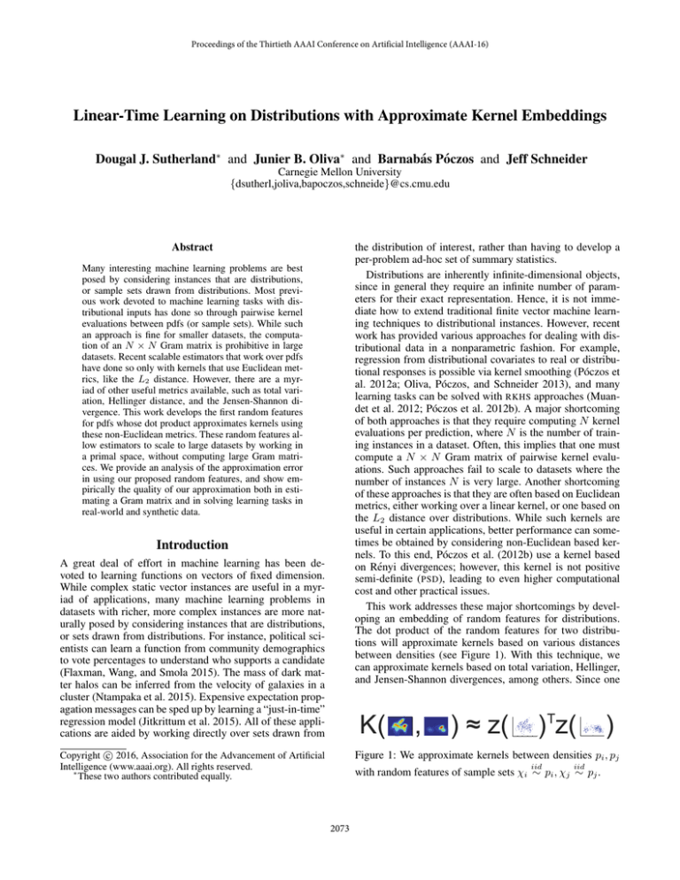
The dot product of the random features for two distributions will approximate kernels based on various distances
between densities (see Figure 1). With this technique, we
can approximate kernels based on total variation, Hellinger,
and Jensen-Shannon divergences, among others. Since one
Abstract
Many interesting machine learning problems are best
posed by considering instances that are distributions,
or sample sets drawn from distributions. Most previous work devoted to machine learning tasks with distributional inputs has done so through pairwise kernel
evaluations between pdfs (or sample sets). While such
an approach is fine for smaller datasets, the computation of an N × N Gram matrix is prohibitive in large
datasets. Recent scalable estimators that work over pdfs
have done so only with kernels that use Euclidean metrics, like the L2 distance. However, there are a myriad of other useful metrics available, such as total variation, Hellinger distance, and the Jensen-Shannon divergence. This work develops the first random features
for pdfs whose dot product approximates kernels using
these non-Euclidean metrics. These random features allow estimators to scale to large datasets by working in
a primal space, without computing large Gram matrices. We provide an analysis of the approximation error
in using our proposed random features, and show empirically the quality of our approximation both in estimating a Gram matrix and in solving learning tasks in
real-world and synthetic data.
Introduction
A great deal of effort in machine learning has been devoted to learning functions on vectors of fixed dimension.
While complex static vector instances are useful in a myriad of applications, many machine learning problems in
datasets with richer, more complex instances are more naturally posed by considering instances that are distributions,
or sets drawn from distributions. For instance, political scientists can learn a function from community demographics
to vote percentages to understand who supports a candidate
(Flaxman, Wang, and Smola 2015). The mass of dark matter halos can be inferred from the velocity of galaxies in a
cluster (Ntampaka et al. 2015). Expensive expectation propagation messages can be sped up by learning a “just-in-time”
regression model (Jitkrittum et al. 2015). All of these applications are aided by working directly over sets drawn from
c 2016, Association for the Advancement of Artificial
Copyright Intelligence (www.aaai.org). All rights reserved.
∗
These two authors contributed equally.
Figure 1: We approximate kernels between densities pi , pj
iid
iid
with random features of sample sets χi ∼ pi , χj ∼ pj .
2073
may work over the primal space induced by the random features there is no need to compute a Gram matrix; thus, one
will be able to use these kernels while still scaling to datasets
with a large number of instances using primal-space techniques. We provide an approximation bound for the embeddings, and demonstrate the efficacy of the embeddings on
both real-world and synthetic data. To the best of our knowledge, this work provides the first non-discretized embedding
for non-L2 kernels for probability density functions.
whose random kitchen sink (RKS) embedding approximates
shift-invariant kernels by sampling their Fourier transform.
A related line of
considers additive kernels of the
work
form K(x, y) =
j=1 κ(xj , yj ), usually defined on R≥0
(e.g. histograms). Maji and Berg (2009) embed the inter
section kernel j=1 min(xj , yj ) via step functions. Vedaldi
and Zisserman (2010) allow any homogeneous κ, so that
κ(tx, ty) = t κ(x, y), providing embeddings for histogram
kernels such as the additive χ2 kernel and Jensen-Shannon
divergence. Their embedding uses the same fundamental result of Fuglede (2005) as ours; we expand to the continuous
rather than the discrete case. Vempati et al. (2010) later apply RKS embeddings for generalized RBF kernels (1).
For embedding kernels on spaces other than R , the RKS
embedding extends naturally to locally compact abelian
groups (Li, Ionescu, and Sminchisescu 2010). Oliva et
al. (2014) embedded an L2 estimate between continuous
densities via orthonormal basis functions. MMK also has a
simple embedding when the base kernel k is embeddable
(Flaxman, Wang, and Smola 2015; Jitkrittum et al. 2015;
Lopez-Paz et al. 2015; Sutherland and Schneider 2015).
Related Work
The two main lines of relevant research are the development
of kernels on probability distributions and explicit approximate embeddings for scalable kernel learning.
Learning on distributions In computer vision, the popular “bag of words” model (Leung and Malik 2001) represents a distribution by quantizing it onto codewords (usually
by k-means on points from all sets), then compares those
histograms with some kernel (often exponentiated χ2 ).
Another approach estimates a distance between distributions, often the L2 distance or Kullback-Leibler (KL)
divergence, parametrically (Jaakkola and Haussler 1998;
Moreno, Ho, and Vasconcelos 2003; Jebara, Kondor, and
Howard 2004) or nonparametrically (Sricharan, Wei, and
Hero 2013; Krishnamurthy et al. 2014). The distance can
then be used in kernel smoothing (Póczos et al. 2012a; Oliva,
Póczos, and Schneider 2013) or Mercer kernels (Moreno,
Ho, and Vasconcelos 2003; Kondor and Jebara 2003; Jebara,
Kondor, and Howard 2004; Póczos et al. 2012b).
These approaches can be powerful, but usually require
computing an N × N matrix of kernel evaluations, which
can be infeasible for large datasets. The use of divergences
in Mercer kernels faces an additional challenge, which is that
the estimated Gram matrix may not be PSD, due to estimation error or because some divergences in fact do not induce
a PSD kernel. In general this must be remedied by altering
the Gram matrix a “nearby” PSD one. Typical approaches
involve eigendecomposing the Gram matrix, which usually
costs O(N 3 ) computation and also presents challenges for
traditional inductive learning, where the test points are not
known at training time (Chen et al. 2009).
One way to alleviate the scaling problem is the Nyström
extension (Williams and Seeger 2001), in which some
columns of the Gram matrix are used to estimate the remainder. In practice, one frequently must compute many
columns, and methods to make the result PSD are known
only for mildly-indefinite kernels (Belongie et al. 2002).
Another approach is to represent a distribution by its mean
RKHS embedding under some kernel k. The RKHS inner
product is known as the mean map kernel (MMK), and the
distance the maximum mean discrepancy (MMD) (Gretton et
al. 2009; Muandet et al. 2012; Szabó et al. 2015). When k is
the RBF kernel, the MMK estimate is proportional to an L2
inner product between Gaussian kernel density estimates.
Embedding Information Theoretic Kernels
For a broad class of distributional distances d, including
many common and useful information theoretic divergences,
we consider generalized RBF kernels of the form
(1)
K(p, q) = exp − 2σ1 2 d2 (p, q) ,
for pdfs p, q: [0, 1] → R≥0 . We construct features z(A(·))
such that K(p, q) ≈ z(A(p))T z(A(q)) as follows:
Embedding HDDs into L2 We define a random function ψ
such that d(p, q) ≈ ψ(p) − ψ(q), where ψ(p) is a function from [0, 1] to R2M . Thus the metric space of densities with distance d is approximately embedded into the
metric space of 2M -dimensional L2 functions.
Finite Embeddings of L2 We use orthonormal basis functions to approximately embed smooth L2 functions into
finite vectors in R|V | . Combined with the previous step,
we obtain features A(p) ∈ R2M |V | such that d is approximated by Euclidean distances between the A(·) features.
Embedding RBF Kernels into RD We use the RKS embedding z(·) so that inner products between z(A(·)) features,
in RD , approximate K(p, q).
We can thus use the powerful kernel K without needing to
compute an expensive N × N Gram matrix.
Homogeneous Density Distances (HDDs)
We consider kernels based on metrics which we term homogeneous density distances (HDDs):
κ(p(x), q(x)) dx,
(2)
d2 (p, q) =
[0,1]
where κ(x, y) : R+ × R+ → R+ is a negative-type kernel,
i.e. a squared Hilbertian metric, and κ(tx, ty) = tκ(x, y) for
all t > 0. Table 1 shows a few important instances. Note we
assume the distributions are supported within [0, 1] .
Approximate embeddings Interest in approximate kernel embeddings was spurred by Rahimi and Recht (2007),
2074
Name
JS
2
κ(p(x), q(x))
1
r∈{p,q} 2 r(x) log
1
2
H
TV
2r(x)
p(x)+q(x)
2
p(x) − q(x)
|p(x) − q(x)|
dμ(λ)
Finite Embeddings of L2
dλ
cosh(πλ)(1+λ2 )
1
2
If densities p and q are smooth, then the L2 metric between
the pλ and qλ functions may be well approximated using
projections to basis functions. Suppose that {ϕi }i∈Z is an
orthonormal basis for L2 ([0, 1]); then we can construct an
orthonormal basis for L2 ([0, 1] ) by the tensor product:
δ(λ = 0) dλ
dλ
2
1
π 1+4λ2
Table 1: Squared HDDs. JS is Jensen-Shannon divergence;
H is Hellinger distance; TV is total variation distance.
{ϕα }α∈Z
∀f ∈ L2 ([0, 1] ), f (x) =
aα (f ) ϕα (x)
d2 (p, q) ≈ ψ(p) − ψ(q)2
≈
R≥0
Let Z = μ(R≥0 ) and cλ = (− 12 + iλ)/( 12 + iλ); then
M
1 a(pR
a(qλRj )2 + a(pIλj ) − a(qλI j )2
λj ) − M j=1
= A(p) − A(q)2
2
κ(x, y) = Eλ∼ Zμ |gλ (x) − gλ (y)|
√
1
where gλ (x) = Zcλ (x 2 +iλ − 1).
We can approximate the expectation with an empirical
iid
mean. Let λj ∼ Zμ for j ∈ {1, . . . , M }; then
where A : L2 ([0, 1] ) → R2M |V | has A(p) given by
1 R
√
a(pλ1 ), . . . , a(pR
a(pIλ1 ), . . . , a(pIλM ) .
λM ), M
(5)
(6)
a(pIλ ) shortly.
We will discuss how to estimate a(pR
λ ), |gλj (x) − gλj (y)|2 .
Embedding RBF Kernels into RD
The A features approximate the HDD (2) in R2M |V | ; thus
applying the RKS embedding (Rahimi and Recht 2007) to
the A features will approximate our generalized RBF kernel
(1). The RKS embedding is1 z : Rm → RD such that for
D/2 iid
fixed {ωi }i=1 ∼ N (0, σ −2 Im ) and for each x, y ∈ Rm :
2
z(x)T z(y) ≈ exp − 2σ1 2 x − y , where
2
sin(ω1T x), cos(ω1T x), . . . .
(7)
z(x) = D
j=1
Hence, using R, I to denote the real and imaginary parts,
d2 (p, q) is equal to:
κ(p(x), q(x)) dx
[0,1]
=
Eλ∼ Zμ |gλ (p(x)) − gλ (q(x))|2 dx
[0,1]
M 2
1 ≈
R(gλj (p(x))) − R(gλj (q(x)))
M j=1 [0,1]
2 dx
+ I(gλj (p(x))) − I(gλj (q(x)))
= ψ(p) − ψ(q)2 ,
ϕαi (xi ), x ∈ [0, 1] ,
and aα (f ) = ϕα , f = [0,1] ϕα (t) f (t) dt ∈ R. Let V ⊂
Z be an appropriately chosen finite set of indices. If f, f ∈
L2 ([0, 1] ) are smooth and a(f ) = (aα1 (f ), . . . , aα|V | (f )),
then f −f 2 ≈ a(f )−a(f )2 . Thus we can approximate
d2 as the squared distance between finite vectors:
Fuglede (2005) shows that κ corresponds to a bounded measure μ(λ), as in Table 1, with
1
1
κ(x, y) =
|x 2 +iλ − y 2 +iλ |2 dμ(λ).
(3)
1
M
α∈Z
Embedding HDDs into L2
κ(x, y) ≈
ϕα (x) =
i=1
We then use these distances in a generalized RBF kernel
(1). d is a Hilbertian metric (Fuglede 2005), so K is positive
definite (Haasdonk and Bahlmann 2004). Note we use the
√
TV metric, even though TV is itself a metric.
Below we expound on the embeddings used to construct
features z(A(·)) such that K(p, q) ≈ z(A(p))T z(A(q)).
M
where
Thus we can approximate the HDD kernel (1) as:
1
K(p, q) = exp − 2 d2 (p, q)
2σ
1
≈ exp − 2 A(p) − A(q)2
2σ
(4)
where [ψ(p)](x) is given by
1 R
I
I
√
pλ1 (x), . . . , pR
λM (x), pλ1 (x), . . . , pλM (x) ,
M
≈ z(A(p))T z(A(q)).
(8)
Finite Sample Estimates
I
defining pR
λj (x) = R(gλj (p(x))), pλj (x) = I(gλj (p(x))).
Hence, the HDD between densities p and q is approximately
the L2 distance from ψ(p) to ψ(q), where ψ maps a function
f : [0, 1] → R to a vector-valued function ψ(f ) : [0, 1] →
R2M of λ functions. M can typically be quite small, since
the kernel it approximates is one-dimensional.
Our final approximation for HDD kernels (8) depends on integrals of densities p and q. In practice, we are unlikely to
directly observe an input density, but even given a pdf p, the
1
There are two versions of the embedding in common use, but
this one is preferred (Sutherland and Schneider 2015).
2075
Then, for any εRKS + σk1√e (εKDE + ελ + εtail + εint ) ≤ ε,
the probability of the error exceeding ε is at most:
2 exp −Dε2RKS + 2 exp −M ε4λ /(8Z 2 ) + δ
4
εKDE n2β/(2β+)
−1
+ 2C
+ 2M 1 − μ [0, utail )
4 log n
⎛
2 ⎞
2
1 + εint /(8 |V | Z) − 1 ⎠
√ ∗
+ 8M |V | exp ⎝− 12 ne
ρ +1
integrals that make up the elements of A(p) are not readily
computable. We thus first estimate the density as p̂, e.g. with
kernel density estimation (KDE), and estimate A(p) as A(p̂).
Recall that the elements of A(p̂) are:
aα (p̂Sλj ) =
ϕα (t) p̂Sλj (t) dt
(9)
[0,1]
where j ∈ {1, . . . , M }, S ∈ {R, I}, α ∈ V . In lower dimensions, we can approximate (9) with simple Monte Carlo
iid
e
numerical integration. Choosing {ui }ni=1
∼ Unif([0, 1] ):
âα (p̂Sλj )
ne
1 =
ϕα (ui ) p̂Sλj (ui ),
ne i=1
where utail
(10)
The bound decreases when the function is smoother
or lower-dimensional (), or when
(larger β, γ̂; smaller L)
we observe more samples (n). Using more projection coefficients (higher t or smaller s, giving higher |V |) improves the
approximation but makes numerical integration more difficult. Likewise, taking more samples from μ (higher M )
improves that approximation, but increases the number of
functions to be approximated and numerically integrated.
For the proof and further details, see the appendix.2
obtaining Â(p̂). We note that in high dimensions, one may
use any high-dimensional density estimation scheme (e.g.
Lafferty, Liu, and Wasserman 2012) and estimate (9) with
MCMC techniques (e.g. Hoffman and Gelman 2014).
Summary and Complexity
The algorithm for computing features {z(A(pi ))}N
i=1 for
N
a set of distributions {pi }N
,
given
sample
sets
{χ
i }i=1
i=1
(i)
iid
i
where χi = {Xj ∈ [0, 1] }nj=1
∼ pi , is thus:
iid
Numerical Experiments
Throughout these experiments we use M = 5, |V | = 10
(selected as rules of thumb; larger values did not improve
performance), and use a validation set (10% of the training
set) to choose bandwidths for KDE and the RBF kernel as
well as model regularization parameters. Except in the scene
classification experiments, the histogram methods used 10
bins per dimension; performance with other values was not
better. The KL estimator used the fourth nearest neighbor.
We evaluate RBF kernels based on various distances. First,
we try our JS, Hellinger, and TV embeddings.
We compare
to
L2 kernels as in Oliva et al. (2014): exp − 2σ1 2 p − q22 ≈
z(a(p̂))T z(a(q̂)) (L2). We also try the MMD distance (Muandet et al. 2012) with
approximate kernel embeddings:
q) ≈ z (z̄(p̂))T z (z̄(q̂)), where z̄ is
exp − 2σ1 2 MMD(p,
n
the mean embedding z̄(p̂) = n1 i=1 z(Xi ) (MMD). We further compare to RKS with histogram JS embeddings (Vempati et al. 2010) (Hist JS); we also tried χ2 embeddings, but
their performance was quite similar. We finally try the full
Gram matrix approach of Póczos et al. (2012b) with the KL
estimator of Wang, Kulkarni, and Verdú (2009) in an RBF
kernel (KL), as did Ntampaka et al. (2015).
iid
1. Draw M scalars λj ∼
and D/2 vectors ωr ∼
N (0, σ −2 I2M |V | ), in O(M |V | D) time.
2. For each of the N input distributions i:
(a) Compute a kernel density estimate from χi , p̂i (uj ) for
each uj in (10), in O(ni ne ) time.
(b) Compute Â(p̂i ) using a numerical integration estimate
as in (10), in O(M |V | ne ) time.
(c) Get the RKS features, z(Â(p̂i )), in O(M |V | D) time.
Supposing each ni n, this process takes a total of
O (N nne + N M |V | ne + N M |V | D) time. Taking |V | to
be asymptotically O(n), ne = O(D), and M = O(1)
for simplicity, this is O(N nD) time, compared to about
O(N 2 n log n+N 3 ) for the methods of Póczos et al. (2012b)
and O(N 2 n2 ) for Muandet et al. (2012).
μ
Z
γ̂
s 2
= max 0, 8Mρ∗tL2 4 4−4
εtail − 14 .
γ̂
Theory
We bound Pr K(p, q) − z(Â(p̂))T z(Â(q̂)) ≥ ε for two
fixed densities p and q by considering each source of error:
kernel density estimation (εKDE ); approximating μ(λ) with
M samples (ελ ); truncating the tails of the projection coefficients (εtail ); Monte Carlo integration (εint ); and the RKS
embedding (εRKS ).
We need some smoothness assumptions on p and q: that
they are members of a periodic Hölder class Σper (β, Lβ ),
that they are bounded below by ρ∗ and above by ρ∗ , and that
with probatheir kernel density estimates are in Σper (γ̂, L)
bility at least 1 − δ. We use a suitable form of kernel density
estimation, to obtain a uniform error bound with a rate based
on the function C −1 (Giné and Guillou 2002). We use the
Fourier basis and choose V = {α ∈ Z | j=1 |αj |2s ≤ t}
for parameters 0 < s < γ̂, t > 0.
Gram Matrix Estimation
We first illustrate that our embedding, using the parameter
selections as above, can approximate the Jensen-Shanon kernel well. We compare three different approaches to estimating K(pi , pj ) = exp(− 2σ1 2 JS(pi , pj )). Each approach uses
kernel density estimates p̂i . The estimates are compared on
a dataset of N = 50 random GMM distributions {pi }N
i=1 and
(i)
iid
samples of size n = 2 500: χi = {Xj ∈ [0, 1]2 }nj=1 ∼ pi .
See the appendix for more details.
2
2076
cs.cmu.edu/∼joliva/papers/joliva aaai16 supp.pdf
form the histogram kernel, especially with |χi | = 200, and
the KL kernel. Note that fitting mixtures with EM and selecting a number of components using AIC (Akiake 1973) or
BIC (Schwarz 1978) performed much worse than regression;
only AIC with |χi | = 800 outperformed the best constant
predictor of 5.5. Linear versions of the L2 and MMD kernels
were also no better than the constant predictor.
The HDD embeddings were more computationally expensive than the other embeddings, but much less expensive
than the KL kernel, which grows at least quadratically in
the number of distributions. Note that the histogram embeddings used an optimized C implementation (Vedaldi and
Fulkerson 2008), as did the KL kernel3 , while the HDD embeddings used a simple Matlab implementation.
The first approach approximates JS based on empirical estimates of entropies E log p̂i . The second approach estimates
JS as the Euclidean distance of vectors of projection coefficients (5) : JSpc (pi , pj ) = Â(p̂i ) − Â(p̂j )2 . For these first
two approaches we compute the pairwise kernel evaluations
1
in the Gram matix as Gent
ij = exp(− 2σ 2 JSent (pi , pj )), and
pc
1
Gij = exp(− 2σ2 JSpc (pi , pj )) using their respective approximations for JS. Lastly, we directly estimate the JS kernel with dot products of our random features (8): Grks
ij =
T
z(Â(p̂i )) z(Â(p̂j )), with D = 7 000.
Figure 2 shows the
N 2 true pairwise kernel
values versus the afore
mentioned
estimates.
Quantitatively, the en
tropy method obtained
a squared correlation
!"
#$
to the true kernel value
%#$
2
of Rent = 0.981; using
the A features with an
exact kernel yielded Figure 2: Estimating RBF with
2
Rpc
= 0.974; adding JS divergence.
RKS embeddings gave
2
Rrks
= 0.966. Thus our method’s estimates are nearly as
good as direct estimation via entropies, while allowing us to
work in primal space and avoid N × N Gram matrices.
Image Classification
As another example of the performance of our embeddings,
we now attempt to classify images based on their distributions of pixel values. We took the “cat” and “dog” classes
from the CIFAR -10 dataset (Krizhevsky and Hinton 2009),
and represented each 32 × 32 image by a set of triples
(x, y, v), where x and y are the position of each pixel in the
image and v the pixel value after converting to grayscale.
The horizontal reflection of the image was also included, so
each sample set χi ⊂ R3 had |χi | = 2 048. This is certainly
not the best representation for these images; rather, we wish
to show that given this simple representation, our HDD kernels perform well relative to the other options.
We used the same kernels as above in an SVM classifier from LIBLINEAR (Fan et al. 2008, for the embeddings)
or LIBSVM (Chang and Lin 2011, for the KL kernel), with
D = 7 000. Figure 5 shows computation time and accuracy
on the standard test set (of size 2K) with 2.5K, 5K, and 10K
training images. Our JS and Hellinger embedding approximately match the histogram JS embedding in accuracy here,
while our TV embedding beats histogram JS; all outperform
L2 and MMD. We could only run the KL kernel for the 2.5K
training set size; its accuracy was comparable to the HDD
and histogram embeddings, at far higher computational cost.
Estimating the Number of Mixture Components
We will now illustrate the efficacy of HDD random features
in a regression task; following Oliva et al. (2014), we estimate the number of components from a mixture of truncated
Gaussians. We generate the distributions as follows: Draw
the number of components Yi for the ith distribution as Yi ∼
(i)
Unif{1, . . . , 10}. For each component select a mean μk ∼
(i)
(i) (i) (i)T
(i)
Unif[−5, 5]2 and covariance Σk = ak Ak Ak + Bk ,
(i)
(i)
where a ∼ Unif[1, 4], Ak (u, v) ∼ Unif[−1, 1], and Bk is
(i)
a diagonal 2 × 2 matrix with Bk (u, u) ∼ Unif[0, 1]. Then
weight each component equally in the mixture. Given a sample χi , we predict the number of components Yi . An example distribution and sample are shown in Figure 3; predicting
the number of components is difficult even for humans.
Scene Classification
Modern computer vision classification systems typically
consist of a deep network with several convolutional and
pooling layers to extract complex features of input images,
followed by one or two fully-connected classification layers.
The activations are of shape n × h × w, where n is the number of filters; each unit corresponds to an overlapping patch
of the original image. We can thus treat the final pooled activations as a sample of size hw from an n-dimensional distribution, similarly to how Póczos et al. (2012b) and Muandet
et al. (2012) used SIFT features from image patches. Wu,
Gao, and Liu (2015) set accuracy records on several scene
classification datasets with a particular ad-hoc method of extracting features from distributions (D3); we compare to our
more principled alternatives.
We consider the Scene-15 dataset (Lazebnik, Schmid, and
Ponce 2006), which contains 4 485 natural images in 15
Figure 3: A GMM and 200 points drawn from it.
Figure 4 presents results for predicting with ridge regression the number of mixture components Yi , given a varying
number of sample sets χi , with |χi | ∈ {200, 800}; we use
D = 5 000. The HDD-based kernels achieve substantially
lower error than the L2 and MMD kernels. They also outper-
3
2077
github.com/dougalsutherland/skl-groups/
3
10 3
10
2
10 2
10
1
Time (cpu-hours)
Time (cpu-hours)
10
KL with kNN
10
KL with kNN
1
TV
TV
JS
JS
10
Hellinger
0
L2
Hist JS
1.35
1.4
1.45
1.5
RMSE
10
MMD
Hist JS
0
1.35
1.55
Hellinger
1.4
(a) Samples of size 200.
MMD
L2
1.45
RMSE
1.5
1.55
(b) Samples of size 800.
Figure 4: Error and computation time for estimating the number of mixture components. The three points on each line correspond to training set sizes of 4K, 8K, and 16K; error is on the fixed test set of size 2K. Note the logarithmic scale on the time
axis. The KL kernel for |χi | = 800 with 16K training sets was too slow to run. AIC-based predictions achieved RMSEs of 2.7
(for 200 samples) and 2.3 (for 800); BIC errors were 3.8 and 2.7; a constant predictor of 5.5 had RMSE of 2.8.
93%
92%
80
KL
70
91%
Time (cpu-hours)
60
50
90%
10
40
20
TV
50
Hellinger
JS
88%
10
MMD
Hist JS
0
0.31
25
89%
30
0.32
0.33
0.34
Error
0.35
L2
0.36
0.37
0.38
87%
Figure 5: Misclassification rate and computation time for classifying CIFAR -10 cats versus dogs. The three points on each
line show training set sizes of 2.5K, 5K, and 10K; error is on
the fixed test set of size 2K. Note the linear scale for time. The
KL kernel was too slow to run for 5 K or 10 K training points.
D3
L2
JS
TV
Hel
HDDs
1
2σ
σ
2σ
MMD
Hist JS
Figure 6: Mean and standard deviation of accuracies on the
Scene-15 dataset in 10 random splits. The left, black lines use
Â(·) features; the right, blue lines show z(Â(·)) features. MMD
methods vary bandwidth are relative to σ, the median of pairwise distances; histogram methods vary the number of bins.
match or beat MMD and substantially outperform D3, L2 ,
and the histogram embeddings.
location categories, and follow Wu, Gao, and Liu in extracting features from the last convolutional layer of the
imagenet-vgg-verydeep-16 model (Simonyan and
Zisserman 2015). We replace that layer’s rectified linear activations with sigmoid squashing to [0, 1].4 hw ranges from
400 to 1 000. There are 512 filter dimensions; we concatenate features Â(p̂i ) extracted from each independently.
We train on the standard for this dataset of 100 images
from each class (1500 total) and test on the remainder; Figure 6 shows results. We did not include spatial information; still, we match the best prior published performance of
91.59 ± 0.48, trained on a large scene classification dataset
(Zhou et al. 2014). Adding spatial information brought the
D3 method to about 92% accuracy; their best hybrid method
obtained 92.9%. With these features, however, our methods
Discussion
This work presents the first nonlinear embedding of density
functions for quickly computing HDD-based kernels, including kernels based on the popular total variation, Hellinger
and Jensen-Shanon divergences. Nonparametric uses of kernels with these divergences previously necessitated the computation of a large N ×N Gram matrix, prohibiting their use
in large datasets. Our embeddings allow one to work in a primal space while using information theoretic kernels. We analyze the approximation error of our embeddings, and show
their quality on several synthetic and real-world datasets.
Acknowledgements
4
We used piecewise-linear weights before the sigmoid function
such that 0 maps to 0.5, the 90th percentile of the positive observations maps to 0.9, and the 10th percentile of the negative observations to 0.1, for each filter.
This work was funded in part by NSF grant IIS1247658 and
by DARPA grant FA87501220324. DJS is also supported by
a Sandia Campus Executive Program fellowship.
2078
References
Lopez-Paz, D.; Muandet, K.; Schölkopf, B.; and Tolstikhin, I.
2015. Towards a learning theory of causation. ICML.
Maji, S., and Berg, A. C. 2009. Max-margin additive classifiers
for detection. In ICCV.
Moreno, P. J.; Ho, P. P.; and Vasconcelos, N. 2003. A KullbackLeibler divergence based kernel for SVM classification in multimedia applications. In NIPS.
Muandet, K.; Fukumizu, K.; Dinuzzo, F.; and Schölkopf, B.
2012. Learning from distributions via support measure machines. In NIPS.
Ntampaka, M.; Trac, H.; Sutherland, D. J.; Battaglia, N.;
Póczos, B.; and Schneider, J. 2015. A machine learning approach for dynamical mass measurements of galaxy clusters.
The Astrophysical Journal 803(2):50.
Oliva, J. B.; Neiswanger, W.; Póczos, B.; Schneider, J.; and
Xing, E. 2014. Fast distribution to real regression. In AISTATS.
Oliva, J. B.; Póczos, B.; and Schneider, J. 2013. Distribution to
distribution regression. In ICML.
Póczos, B.; Rinaldo, A.; Singh, A.; and Wasserman, L. 2012a.
Distribution-free distribution regression. AISTATS.
Póczos, B.; Xiong, L.; Sutherland, D. J.; and Schneider, J.
2012b. Nonparametric kernel estimators for image classification. In CVPR.
Rahimi, A., and Recht, B. 2007. Random features for largescale kernel machines. In NIPS.
Schwarz, G. 1978. Estimating the dimension of a model. Ann.
Statist. 6(2):461–464.
Simonyan, K., and Zisserman, A. 2015. Very deep convolutional networks for large-scale image recognition. In ICLR.
Sricharan, K.; Wei, D.; and Hero, III, A. O. 2013. Ensemble
estimators for multivariate entropy estimation. IEEE Trans. Inf.
Theory 59:4374–4388.
Sutherland, D. J., and Schneider, J. 2015. On the error of random Fourier features. In UAI.
Szabó, Z.; Gretton, A.; Póczos, B.; and Sriperumbudur, B.
2015. Two-stage sampled learning theory on distributions. AISTATS.
Vedaldi, A., and Fulkerson, B. 2008. VLFeat: An open and
portable library of computer vision algorithms. http://www.
vlfeat.org/.
Vedaldi, A., and Zisserman, A. 2010. Efficient additive kernels
via explicit feature maps. In CVPR.
Vempati, S.; Vedaldi, A.; Zisserman, A.; and Jawahar, C. V.
2010. Generalized RBF feature maps for efficient detection.
In British Machine Vision Conference.
Wang, Q.; Kulkarni, S. R.; and Verdú, S. 2009. Divergence estimation for multidimensional densities via k-nearest-neighbor
distances. IEEE Trans. Inf. Theory 55(5):2392–2405.
Williams, C. K. I., and Seeger, M. 2001. Using the Nyström
method to speed up kernel machines. In NIPS.
Wu, J.; Gao, B.-B.; and Liu, G. 2015. Visual recognition using
directional distribution distance.
Zhou, B.; Lapedriza, A.; Xiao, J.; Torralba, A.; and Oliva, A.
2014. Learning deep features for scene recognition using Places
database. In NIPS.
Akiake, H. 1973. Information theory and an extension of the
maximum likelihood principle. In 2nd Int. Symp. on Inf. Theory.
Belongie, S.; Fowlkes, C.; Chung, F.; and Malik, J. 2002. Spectral partitioning with indefinite kernels using the Nyström extension. In ECCV.
Chang, C.-C., and Lin, C.-J. 2011. LIBSVM: a library for support vector machines. ACM Trans. Intell. Syst. Technol. 2(3):1–
27.
Chen, Y.; Garcia, E. K.; Gupta, M. R.; Rahimi, A.; and Cazzanti, L. 2009. Similarity-based classification: Concepts and
algorithms. JMLR 10:747–776.
Fan, R.-E.; Chang, K.-W.; Hsieh, C.-J.; Wang, X.-R.; and Lin,
C.-J. 2008. LIBLINEAR: A library for large linear classification. JMLR 9:1871–1874.
Flaxman, S. R.; Wang, Y.-x.; and Smola, A. J. 2015. Who
supported Obama in 2012? Ecological inference through distribution regression. In KDD, 289–298.
Fuglede, B. 2005. Spirals in Hilbert space: With an application
in information theory. Exposition. Math. 23(1):23–45.
Giné, E., and Guillou, A. 2002. Rates of strong uniform consistency for multivariate kernel density estimators. Ann. Inst. H.
Poincaré Probab. Statist. 38(6):907–921.
Gretton, A.; Fukumizu, K.; Harchaoui, Z.; and Sriperumbudur,
B. K. 2009. A fast, consistent kernel two-sample test. In NIPS.
Haasdonk, B., and Bahlmann, C. 2004. Learning with distance
substitution kernels. In Pattern Recognition: 26th DAGM Symposium, 220–227.
Hoffman, M. D., and Gelman, A. 2014. The No-U-Turn
Sampler: Adaptively setting path lengths in Hamiltonian Monte
Carlo. JMLR 15(1):1593–1623.
Jaakkola, T., and Haussler, D. 1998. Exploiting generative
models in discriminative classifiers. In NIPS.
Jebara, T.; Kondor, R.; and Howard, A. 2004. Probability product kernels. JMLR 5:819–844.
Jitkrittum, W.; Gretton, A.; Heess, N.; Eslami, S.; Lakshminarayanan, B.; Sejdinovic, D.; and Szabó, Z. 2015. Kernelbased just-in-time learning for passing expectation propagation
messages. UAI.
Kondor, R., and Jebara, T. 2003. A kernel between sets of
vectors. In ICML.
Krishnamurthy, A.; Kandasamy, K.; Poczos, B.; and Wasserman, L. 2014. Nonparametric estimation of Rényi divergence
and friends. In ICML.
Krizhevsky, A., and Hinton, G. 2009. Learning multiple layers
of features from tiny images. University of Toronto, Tech. Rep.
Lafferty, J.; Liu, H.; and Wasserman, L. 2012. Sparse nonparametric graphical models. Statistical Science 27(4):519–537.
Lazebnik, S.; Schmid, C.; and Ponce, J. 2006. Beyond bags
of features: Spatial pyramid matching for recognizing natural
scene categories. In CVPR.
Leung, T., and Malik, J. 2001. Representing and recognizing
the visual appearance of materials using three-dimensional textons. IJCV 43.
Li, F.; Ionescu, C.; and Sminchisescu, C. 2010. Random Fourier
approximations for skewed multiplicative histogram kernels. In
Pattern Recognition: DAGM, 262–271.
2079