Proceedings of the Thirtieth AAAI Conference on Artificial Intelligence (AAAI-16)
Generating CP-Nets Uniformly at Random
Thomas E. Allen
Judy Goldsmith
University of Kentucky
Lexington, Kentucky, USA
teal223@g.uky.edu
University of Kentucky
Lexington, Kentucky, USA
goldsmit@cs.uky.edu
Hayden E. Justice
Nicholas Mattei
Kayla Raines
The Gatton Academy, WKU
Bowling Green, Kentucky, USA
hayden.justice259@topper.wku.edu
Data61 and UNSW
Sydney, Australia
nicholas.mattei@nicta.com.au
University of Kentucky
Lexington, Kentucky, USA
kayla.raines@live.com
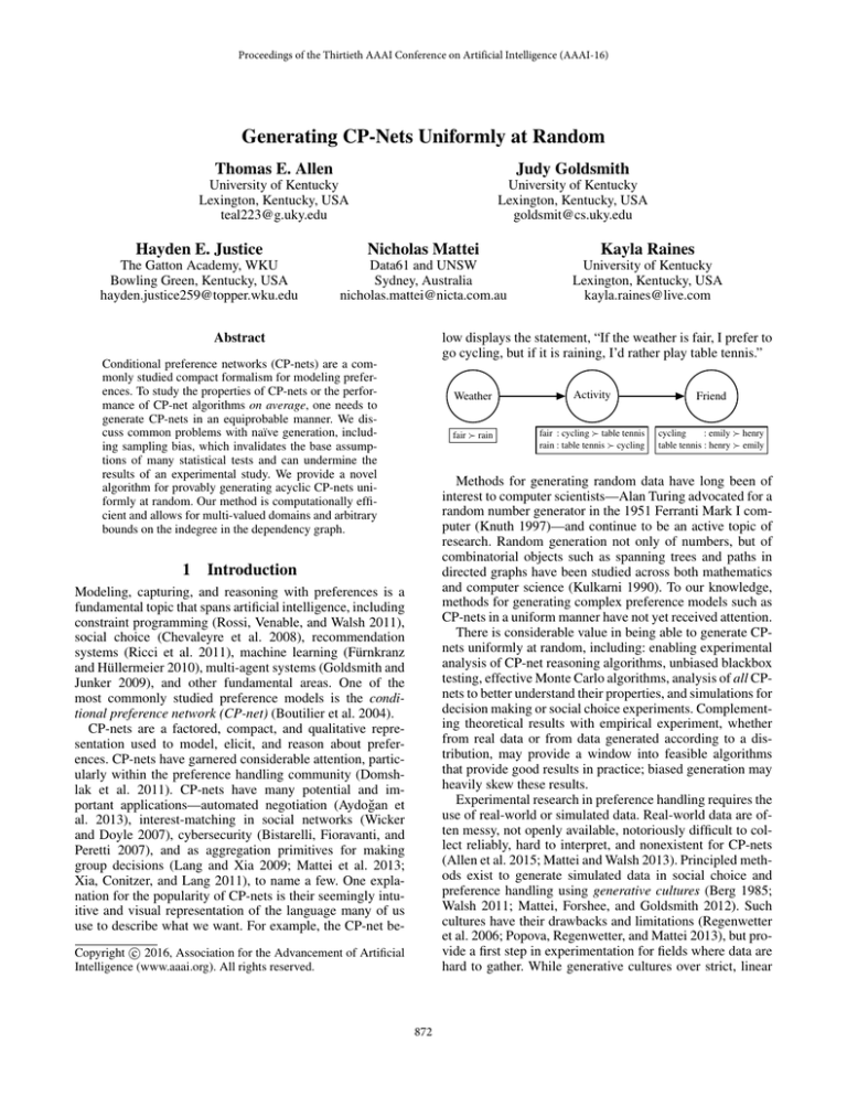
low displays the statement, “If the weather is fair, I prefer to
go cycling, but if it is raining, I’d rather play table tennis.”
Abstract
Conditional preference networks (CP-nets) are a commonly studied compact formalism for modeling preferences. To study the properties of CP-nets or the performance of CP-net algorithms on average, one needs to
generate CP-nets in an equiprobable manner. We discuss common problems with naı̈ve generation, including sampling bias, which invalidates the base assumptions of many statistical tests and can undermine the
results of an experimental study. We provide a novel
algorithm for provably generating acyclic CP-nets uniformly at random. Our method is computationally efficient and allows for multi-valued domains and arbitrary
bounds on the indegree in the dependency graph.
1
Weather
Activity
Friend
fair rain
fair : cycling table tennis
rain : table tennis cycling
cycling
: emily henry
table tennis : henry emily
Methods for generating random data have long been of
interest to computer scientists—Alan Turing advocated for a
random number generator in the 1951 Ferranti Mark I computer (Knuth 1997)—and continue to be an active topic of
research. Random generation not only of numbers, but of
combinatorial objects such as spanning trees and paths in
directed graphs have been studied across both mathematics
and computer science (Kulkarni 1990). To our knowledge,
methods for generating complex preference models such as
CP-nets in a uniform manner have not yet received attention.
There is considerable value in being able to generate CPnets uniformly at random, including: enabling experimental
analysis of CP-net reasoning algorithms, unbiased blackbox
testing, effective Monte Carlo algorithms, analysis of all CPnets to better understand their properties, and simulations for
decision making or social choice experiments. Complementing theoretical results with empirical experiment, whether
from real data or from data generated according to a distribution, may provide a window into feasible algorithms
that provide good results in practice; biased generation may
heavily skew these results.
Experimental research in preference handling requires the
use of real-world or simulated data. Real-world data are often messy, not openly available, notoriously difficult to collect reliably, hard to interpret, and nonexistent for CP-nets
(Allen et al. 2015; Mattei and Walsh 2013). Principled methods exist to generate simulated data in social choice and
preference handling using generative cultures (Berg 1985;
Walsh 2011; Mattei, Forshee, and Goldsmith 2012). Such
cultures have their drawbacks and limitations (Regenwetter
et al. 2006; Popova, Regenwetter, and Mattei 2013), but provide a first step in experimentation for fields where data are
hard to gather. While generative cultures over strict, linear
Introduction
Modeling, capturing, and reasoning with preferences is a
fundamental topic that spans artificial intelligence, including
constraint programming (Rossi, Venable, and Walsh 2011),
social choice (Chevaleyre et al. 2008), recommendation
systems (Ricci et al. 2011), machine learning (Fürnkranz
and Hüllermeier 2010), multi-agent systems (Goldsmith and
Junker 2009), and other fundamental areas. One of the
most commonly studied preference models is the conditional preference network (CP-net) (Boutilier et al. 2004).
CP-nets are a factored, compact, and qualitative representation used to model, elicit, and reason about preferences. CP-nets have garnered considerable attention, particularly within the preference handling community (Domshlak et al. 2011). CP-nets have many potential and important applications—automated negotiation (Aydoğan et
al. 2013), interest-matching in social networks (Wicker
and Doyle 2007), cybersecurity (Bistarelli, Fioravanti, and
Peretti 2007), and as aggregation primitives for making
group decisions (Lang and Xia 2009; Mattei et al. 2013;
Xia, Conitzer, and Lang 2011), to name a few. One explanation for the popularity of CP-nets is their seemingly intuitive and visual representation of the language many of us
use to describe what we want. For example, the CP-net bec 2016, Association for the Advancement of Artificial
Copyright Intelligence (www.aaai.org). All rights reserved.
872
to a labeled directed acyclic graph. CPT(Xi |Xh = xhk ) denotes all rules of CPT(Xi ) of the form uxhk : i where
xhk ∈ Dom(Xh ), Xh ∈ Pa(Xi ), u ∈ Asst(Pa(Xi )\{Xh }).
We assume here that CPTs are complete, i.e., have rules for
all dm assignments to parents, where m = |Pa (Xi )| is the
indegree of Xi . Since the number of rules is exponential
in m, we make the customary assumption that indegree is
bounded by a small constant, i.e., |Pa (Xi )| ≤ c for all Xi .
orders are well defined in social choice, there is not an analog for preferences over more complex structures such as
CP-nets. To generalize any statistical cultures used in social
choice, we need to be able to generate samples uniformly at
random from a specified set of CP-nets.
A key idea of our method is that the structure of a CPnet is equivalent to a tuple of sets representing the parents
of nodes in the network. We show how to enumerate all
such dagcodes, as these tuples are known, and how to calculate the number of CP-nets—the possible graphs and conditional preference tables (CPTs)—that extend a partial dagcode. The resulting novel recurrence allows us to generate
the graph and CPTs, node by node, such that all acyclic CPnets with a given domain size and bound on indegree are
equiprobable.
We first formalize definitions that we need to discuss CPnets and random generation, highlighting two problems—
bias and degeneracy—that result from commonly used naı̈ve
generation methods. We show how to encode and count the
dependency graphs. We next show how to avoid degeneracy
in the CPTs and extend the recurrence to count all combinations of CPTs that a partially specified CP-net can have. Finally, we bring these results together to create an algorithm
that samples the space of CP-nets uniformly.
2
3
If one wants to generate CP-nets without regard for the resulting distribution, many simple random methods exist. For
example, initialize a CP-net with n nodes, no edges, and
empty CPTs; choose a random subset of pairs (Xh , Xi ),
h < i, inserting an edge from each Xh to Xi ; generate a
CPT for each Xi with d|Pa(Xi )| rules, each a random permutation of the d values of Xi ; and randomly permute the n
labels. We suspect that something along these lines is meant
when we read in papers, “We generated 1000 CP-nets at random.” However, the resulting distribution is biased statistically, and this bias calls into question the validity of experiments and the ensuing analysis of algorithms and methods.
To understand this bias, consider the following dependency graphs and their associated CP-net count (for d = 2).
Preliminaries
E
A preference relation is a partial order (a reflexive, antisymmetric, transitive binary relation) on a set of outcomes
O, where o o means o is preferred to o . We assume O is
finite and can be factored into variables V = {X1 , . . . , Xn }
with associated domains Dom(Xi ) = {xi1 , . . . , xid } such
that O = Dom(X1 ) × · · · × Dom(Xn ).1 We assume domain sizes are homogeneous; i.e., |Dom (Xi )| = d for all
Xi ∈ V. When a variable is constrained to exactly one
value of its domain, we say the value has been assigned to
it. We designate by Asst(U) the set of all assignments to
U ⊆ V. An assignment to all variables U = V designates a
unique outcome o ∈ O. We denote by uxik the combination
of u ∈ Asst(U) and xik ∈ Dom(Xi ), where U ∩ {Xi } = ∅.
The symbols and \ denote set complementation and subtraction; e.g., U ≡ V \ U. For d-ary variables the total outcome space is |O| = dn ; i.e., exponential space is required
to store . However, since O is factored, a conditional preference network potentially provides a compact model of .
Definition 1. A CP-net is a directed acyclic graph (DAG)
in which each node Xi ∈ V is labeled with a conditional
preference table for its variable. An edge (Xh , Xi ) indicates
that the preferences over Xi in depend on the value of Xh .
We thus call Xh a parent of Xi . We denote by Pa(Xi ) the set
of all such parents.
Definition 2. A conditional preference table CPT(Xi ) specifies the preferences over node Xi given an assignment to
its parents. Each CPT consists of rules of the form u : i
specifying a linear order on Xi for all u ∈ Asst(Pa(Xi )).
We use the term dependency graph to refer to the graph of
a CP-net apart from its CPTs. The term DAG always refers
1
Naı̈ve Generation, Bias, and Degeneracy
E
B
A
32 CP-nets
D
C
D
A
B
C
1,033,504 CP-nets
Observe that for the chain-shaped graph on the left, there are
just two ways to choose each of the n CPTs such that they
are consistent with the dependency graph. The CPT of root
E could be [e1 e2 ] or [e2 e1 ]. The other nodes, each
of which has only one parent, also have two possibilities for
their CPT; e.g., CPT(A) could be [b1 : a1 a2 , b2 : a2 a1 ] or [b1 : a2 a1 , b2 : a1 a2 ]. However, in the case
of the star-shaped graph on the right, CPT(A ) has d4 = 16
rules, each with d! = 2 possible orderings. In all, over one
million CP-nets have the graph on the right, while only 32
have the graph on the left. Further observe that the ratio of
this imbalance increases with the domain size d. Thus, if
the algorithm above in fact generated the two graphs with
equal likelihood, it would grossly oversample CP-nets with
the first graph, while correspondingly undersampling those
with the second.
However, the naı̈ve algorithm does not even generate the
two DAGs with equal likelihood. Since there are 5! = 120
ways to permute the labels of the first DAG, but only 5 ways
to permute those of the second, the star-shaped DAG on the
right would be generated 24 times as often as the chainshaped DAG on the left. Despite this, the CP-nets in the starshaped case would still be greatly undersampled.
A separate problem, degeneracy, can arise in assigning
the CPTs, regardless of how the DAGs are generated.
The notation follows that of Boutilier et al. (2004).
873
The sets {1} and {1, 3} indicate that one node has parent
X1 and another has parents X1 and X3 ; the third (implicit)
node is a root. The mapping from parent sets to their children can be recovered from DAGCODE - TO -DAG (Alg. 1)
(Steinsky 2003, adapted) working right to left as follows:
A2 = {1, 3} corresponds to the parents of X2 since 2 is
the largest unassigned label not in {1} ∪ {1, 3}. A1 = {1}
corresponds to the parents of X3 since 3 is the largest unassigned label not in {1}. The remaining root node is X1 .
Example 3. Consider the following CP-net.
c1 c2
c 1 d1
c 1 d2
c 2 d1
c 2 d2
: a2
: a2
: a1
: a1
a1
a1
a2
a2
C
A
D
c 1 : d 1 d2
c 2 : d 2 d1
B
a1 d1
a1 d2
a2 d1
a2 d2
: b1
: b1
: b1
: b2
b2
b2
b2
b1
The edge from D to A indicates that the preference over the
values of A depends on the value of D. However, in examining the CPT of A closely, one can observe that the preference over A does not in fact depend on D. It can thus be
represented by the following, simpler CP-net.
c1 c2
c 1 : a2 a1
c 2 : a1 a2
C
A
D
c 1 : d1 d2
c 2 : d2 d1
B
a1 d1
a1 d2
a2 d1
a2 d2
: b1
: b1
: b1
: b2
Observe that a DAG has bounded indegree c iff |Aj | ≤ c
for all Aj in the corresponding dagcode: every node Xi in
the DAG corresponds to the parent set of an element Aj in
the dagcode, with the exception of a root with indegree 0.
Our generation method depends on counting the number
of extensions to a partially specified graph. Consider a partial
encoding A<3 = {1}, {2}, of a graph with n = 4
nodes and bound c = 1 on indegree. Here the
could be
any subset of {1, 2, 3, 4} of cardinality 0 or 1 such that the
resulting dagcode is valid, viz., ∅, {1}, {2}, {3}, or {4}.
Generalizing, let A<j = A1 , . . . , Aj−1 , , . . . , be a
partial dagcode for which only elements A1 through Aj−1
have been specified,
such that for all k, 1 ≤ k < j, Ak ⊂ V ,
V = {1, . . . , n}, | ≤k A | ≤ k, and |Ak | ≤ c.
Algorithm 2 generates all extensions to A<j by recursively combining A<j with each Aj such that the resulting
partial dagcode A<j+1 satisfies the constraints on cardinality and indegree. To generate all DAGs with n nodes and
bound c on indegree, we call A LL -DAG S(n, c, 1, 0, ∅, A<1 ).
b2
b2
b2
b1
Understanding when a CPT is degenerate is crucial to generating CP-nets uniformly at random.
4
Encoding and Counting Graphs
To facilitate unbiased generation, we model the dependency
graphs of CP-nets as dagcodes (Steinsky 2003), inspired by
Prüfer codes for labeled trees (Kreher and Stinson 1999). We
first treat the dagcode as an abstraction and then show how
it relates to the dependency graph.
Definition 4. A dagcode A = A1 , . . . , An−1 is a tuple of
n − 1 subsets
Aj ⊂ {1, . . . , n} that satisfy the cardinality
constraint | k≤j Ak | ≤ j for all j, 1 ≤ j < n.
Observe from Def. 4 that tuples {1}, {1, 3}
and {3}, ∅
are valid dagcodes (n = 3), but {1, 2}, ∅
and ∅, {1, 2, 3}
are not, since each violates the cardinality constraint. Steinsky (2003) proved that dagcodes correspond one-to-one with
DAGs and described efficient algorithms for converting dagcodes to DAGs (see Alg. 1) and vice versa.
Applied to CP-nets, each subset Aj ⊂ {1, . . . , n} in the
dagcode corresponds to the parents of some node Xi in the
dependency graph: i.e., h ∈ Aj =⇒ Xh ∈ Pa(Xi ). Note
that the root node with the smallest label is implicit; informally, it is helpful to consider every dagcode as having an
implicit element A0 ≡ ∅. The order in which the remaining
n − 1 parent sets Pa(Xi ) occur in the dagcode depends on
the order of the child node Xi with respect to other nodes in
the graph and the relative size of node label i, as follows:
1. If Xh is an ancestor of Xi in the DAG, the encoded parent
set Pa(Xh ) is ordered before Pa(Xi ) in the dagcode.
2. If h < i and Xh is neither an ancestor nor a descendant
of Xi , then Pa(Xh ) is ordered before Pa(Xi ).
Example 5. The dagcode {1}, {1, 3}
corresponds to a
DAG with n = 3 nodes depicted below.
Theorem 6. A LL -DAG S generates each DAG exactly once.
Proof. (Sketch.) Since dagcodes are in one-to-one correspondence with DAGs (Steinsky 2003, Cor. 1), it suffices
to show that each dagcode is generated exactly once. For
this we will use the recursion invariant: Each time Line 1
isreached, A<j is valid; that is, for all k, 1 ≤ k < j,
| ≤k A | ≤ k and |Ak | ≤ c. We will show that under this
assumption, Alg. 2 generates each Aj such that the invariant holds for A<j+1 . Base case: Observe that the invariant
holds trivially for the empty dagcode A<1 = , . . . , .
Inductive hypothesis:Assume the invariant holds for A<j ,
1 ≤ j < n. Let U = k<j Ak and q = |U |. Observe that
the invariant will also hold for A<j+1 so long as we choose
Aj ⊂ V such that |U ∪ Aj | ≤ j and |Aj | ≤ c. We can select
each element of Aj either from U or U . Let Aj = S ∪ T ,
where S ⊆ U and T ⊆ U . Let s = |S| and t = |T |; hence,
0 ≤ s ≤ q and 0 ≤ t ≤ n − q. Observe that |U ∪ Aj | ≤ j
iff q + t ≤ j, and |Aj | < c iff s + t ≤ c. Line 3 iterates
over all (s, t) that satisfy these conditions. Lines 4–5, then,
iterate over all Aj = S ∪ T such that the invariant holds for
A<j+1 . Thus each Aj is generated such that A<j+1 is valid.
Furthermore, since no pair (s, t) is ever repeated in the outer
loop and S ∩ T ≡ ∅, no subset Aj = S ∪ T is ever repeated.
Termination: Since j increments with each descent, recursion bottoms out at j = n, and a DAG corresponding to fully
specified dagcode A = A<n is output. After all valid combinations A1 , . . . , An−1 are output, Alg. 2 terminates.
X1
X2
X3
From A LL -DAG S we derive a new recurrence for the
874
DAGCODE - TO -DAG( A )
Input:
dagcode A = A1 , . . . , An−1 A LL -DAG S( n, c, j, q, U, A<j )
Inputs: n
number of nodes
c
bound on indegree
j
index of current element Aj
q
current value of |U |
U
current value of A1 ∪ · · · ∪ Aj−1
A<j partial dagcode
Output: corresponding DAG G
1: n ← length(A) + 1
2: Q ← {1, . . . , n}
3: initialize DAG G with n nodes and no edges
4: for j ← n − 1 downto 1 do
5: i ← max Q \ jk=1 Ak
6: for all h ∈ Aj do
7:
insert edge to Xi from its parent Xh
8: Q ← Q \ {i}
9: output DAG G
1: if j = n then
2: DAGCODE - TO -DAG(A<n ); return
3: for all s, t ≥ 0, s ≤ q, s + t ≤ c, q + t ≤ j do
4: for all S ⊆ U, |S| = s do
5:
for all T ⊆ U , |T | = t do
6:
Aj ← S ∪ T ; include Aj with A<j to form A≤j
7:
A LL -DAG S(n, c, j + 1, q + t, U ∪ Aj , A≤j )
Algorithm 1: Generate a DAG from its dagcode
Algorithm 2: Generate all DAGs that extend dagcode A<j
number of DAGs that is more easily extended to CP-nets
than those of Robinson (1973) and Steinsky (2003).
Let an,c denote the number of DAGs (resp. dagcodes)
with nnodes and bound c on indegree. Let an,c (j, q), where
q = | k<j Ak |, denote the number of extensions to a partial dagcode A<j . That is, an,c (j, q) is the number of ways
to choose the remaining elements Aj , . . . , An−1 such that
the cardinality and indegree constraints are satisfied.
Observe that if variables are binary (d = 2), Fj is a Boolean
function. In that case the values xh1 and xh2 of each parent
Xh can map to 0 and 1 respectively. The two possible linear
orders xi1 xi2 and xi2 xi1 can correspond to the outputs
1 and 0. For example, we can model the degenerate CPT of
node A from Example 3 with the following truth table.
CPT(A)
c 1 d 1 : a 2 a1
c 1 d 2 : a 2 a1
c 2 d 1 : a 1 a2
c 2 d 2 : a 1 a2
Theorem 7. an,c = an,c (1, 0). For j = n, an,c (j, q) = 1;
for all j, 0 < j < n, an,c (j, q) =
qn − q
an,c (j + 1, q + t).
(1)
t
s
In2
0
1
0
1
Out
0
0
1
1
Formally, we say Fj (u) is vacuous in variable uk iff its
output never depends on uk ; i.e., for all u ∈ {0, . . . , d−1}m ,
s≥0, t≥0,
s≤q, s+t≤c,
q+t≤j
Fj (u1 , . . . , uk−1 , 0, uk+1 , . . . , um )
= Fj (u1 , . . . , uk−1 , 1, uk+1 , . . . , um )
= · · · = Fj (u1 , . . . , uk−1 , d − 1, uk+1 , . . . , um ).
Proof. (Sketch.) Base case (j = n): One DAG is generated at Line 2; hence, an,c (n, q) = 1 for all q. Inductive
hypothesis: Assume an,c (j , q ) gives the correct count for
j > j and all q . We will show that the resulting count for
an,c (j, q) is also correct. Observe that, whatever the
size of
set U ⊂ V , the loop at Line 4 iterates over the qs ways
to choose s elements
from U . Similarly, the loop at Line 5
iterates over the n−q
ways to choose t elements from U .
t
Note that the number of DAGs generated in the body of the
outermost loop depends on s and t, which differ on each
iteration. Thus, for all (s, t) as defined in Line 3, we take
the sum of the DAGs generated in the loop body, obtaining
the result given in Eq. 1. Finally, observe that all dagcodes
parameterized by n, c extend the fully unspecified dagcode
A<1 = , . . . , , for which j = 1 and q = 0. Thus,
an,c = an,c (1, 0).
5
In1
0
0
1
1
Function Fj is degenerate if it is vacuous in a variable; otherwise, it is non-degenerate. By extension we say a CPT is
degenerate (resp. vacuous in a parent variable) if function Fj
to which it maps is degenerate (resp. vacuous in an input).
Let φd (m) be the total number of possible CPTs for
a node with m parents, and let ψd (m) be the number of
those that are non-degenerate. First consider binary domains
(d = 2). Since CPTs and Boolean functions are in oneto-one correspondence, φ2 (m) is equivalent to the number
of Boolean functions of m inputs, and ψ2 (m) is equivalent to the number of non-degenerate Boolean functions.
Hu (1968, §2, §10) (cf. Harrison 1965, O’Connor
1997)
m
proved that for Boolean functions φ2 (m) = 22 , ψ2 (m) =
2k
m
m−k m
ψ2 (m)/φ2 (m) = 1.
k=0 (−1)
k 2 , and limm→∞
We now generalize these results to domains of size d > 1.
Counting and Generating the CPTs
Theorem 8. φd (m) = d!d
We can generalize the notion of a degenerate CPT introduced in Section 3 with the help of a bijection with discrete
multi-valued functions. We model each CPT(Xi ) as a function Fj : {0, . . . , d − 1}m → {0, . . . , d! − 1}. The inputs
correspond to the values of the m parents of Xi . The output
corresponds to one of the d! orderings on the domain of Xi .
m
Proof. Each rule of CPT(Xi ) specifies one of d! linear orders of Dom(Xi ). The number of rules is |Asst (Pa(Xi ))| =
dm , where m = |Pa (Xi )|. Since each rule can be assigned
m
independently, φd (m) = d!d .
875
B UILD -CP- NET( A, F )
Input:
A = A1 , . . . , An−1 dagcode defining graph
F = F0 , . . . , Fn−1 cpt-code defining CPTs
Output:
the corresponding CP-net N
1:
2:
3:
4:
5:
6:
7:
8:
9:
10:
11:
A LL -CP- NETS( n, c, d, j, q, U, A<j , F<j )
Inputs: n number of nodes
c bound on indegree
d size of domains
j is the index of current elements Aj , Fj
q = |U |, where U = A1 ∪ · · · ∪ Aj−1
A<j , F<j are the partial dagcode and cpt-code
1: if j = n then
2: B UILD -CP- NET(A<n , F<n ); return
3: for all s, t ≥ 0, s ≤ q, s + t ≤ c, q + t ≤ j do
4: for all S ⊆ U, |S| = s do
5:
for all T ⊆ V \ U, |T | = t do
6:
if j > 0 then
7:
Aj ← S ∪ T ; include Aj with A<j to form A≤j
8:
for all Fj : {0, . . . , d − 1}|Aj | → {0, . . . , d! − 1} do
9:
if Fj is non-degenerate then
10:
A LL -CP- NETS(n, c, d, j+1, q+t, U ∪ Aj , A≤j ,F≤j )
n ← length(A) + 1; Q ← {1, . . . , n}
initialize CP-net N with n nodes, no edges, empty CPTs
for j ← n − 1 downto
1 do
i ← max(Q \ jk=1 Ak )
for all h ∈ Aj do
insert edge to Xi from its parent Xh
construct CPT(Xi ) from Aj , Fj
Q ← Q \ {i}
i ← the only remaining element in Q
construct CPT(Xi ) from F0
output CP-net N
Algorithm 4: Generate all CP-nets that extend A<j
Algorithm 3: Construct CP-net from its encoding
Theorem 9. ψd (m) =
m
k=0 (−1)
m−k m
k
k
d!d .
degenerate. With probability ψd (m)/φd (m), asymptotic to
1, we will obtain a non-degenerate CPT on a given attempt.
Theorem 10. limm→∞ ψd (m)/φd (m) = 1.
(The proofs of Thms. 9 and 10, omitted here, follow those
of Hu (1968) [§2, §10] for Boolean functions.)
6
Generating CP-nets
We can now extend A LL -DAG S (Alg. 2) to generate A LL CP- NETS (Alg. 4). CP-nets with the same dependency graph
differ if any rule of a CPT differs. To generate all combinations of CPTs, we need only introduce a new innermost loop
iterating over the possibilities. Since the dagcode is partial,
we do not yet have all of the information we need to construct the CPT: we know the parents, but not the child to
which they belong. However, we do have enough information to iterate over the corresponding functions Fj , since we
know the number of parents (|Aj | = s + t) and the size (d)
of every domain, so we do that instead. Each Fj is included
in a tuple F = F0 , . . . , Fn−1 that we call a cpt-code. (We
use F<j and F≤j , analogous to A<j and A≤j , for a partial cpt-code.) Since a root node is implicit in the dagcode,
F contains an additional element F0 corresponding to that
node’s CPT, and we invoke Alg. 2 with j = 0 instead of 1.
When j = n, the encoding is complete: A and F fully and
uniquely characterize a CP-net N . We call Alg. 3 (cf. Alg. 1)
to decode it—the DAG from A, the CPTs from F .
Theorems 6 and 7 can similarly be extended to CP-nets.
Let an,c,d denote the number of CP-nets with n nodes,
boundc on indegree, and domains of size d. Let an,c,d (j, q),
q = | k<j Ak |, be the number of those that extend A<j .
Theorem 11. Determining whether a CPT (resp. its corresponding function Fj ) is degenerate can be conducted in
time polynomial in the size of the CPT (resp. domain of Fj ).
Proof. (Sketch.) Recall that a CPT of Xi ∈ V is degenerate if it is vacuous in any parent Xh . It is vacuous in Xh
if CPT(Xi | Xh = xhk ) = CPT(Xi | Xh = xh ) for all xhk ,
xh ∈ Dom(Xh ). Note that we can check the CPT of Xi for
degeneracy using an algorithm with 4 nested loops: 1. Iterate over each Xh ∈ Pa(Xi ) to check whether the CPT is
vacuous in Xh . 2. For each Xh , iterate over the d values of
xhk ∈ Dom(Xh ). 3. For each xhk , 1 < k ≤ d, iterate over
the |Asst (Pa(Xi ))| = d|Pa(Xi )| rules to determine whether
CPT(Xi | Xh = xhk ) = CPT(Xi | Xh = xh1 ) in each case.
4. For each rule uxhk : i , u ∈ Asst(Pa(Xi ) \ {Xh }), iterate over the d values that specify the linear order i on
Xi . Let m denote the number of parents of Xi . Note that the
input is dm+1 , since the CPT has dm rules of length d. The
nested loops require O(mdm+2 ) time. Thus, we can check
for degeneracy in time polynomial in the size of the input.
Moreover, since CPTs of d-ary nodes with m parents correspond one-to-one with functions Fj : {0, . . . , d − 1}m →
{0, . . . , d! − 1}, the proof applies also to the latter.
Theorem 12. Algorithm 4 generates, exactly once, each
CP-net N that extends partial dagcode A<j .
We can leverage these results to generate non-degenerate
CPTs efficiently and uniformly. For tiny values of d and m,
we can choose uniformly from a modest-sized table of nondegenerate functions (e.g., ψ2 (4) = 64594). For larger values, we use rejection sampling, generating a random permutation i for each assignment to parents and repeating this
process in the unlikely event (e.g., < 0.0001 for m > 4 and
very rapidly converging to 0 as m increases) that the result is
Theorem 13. an,c,d = an,c,d (0, 0). For j=n, an,c,d (j, q) =
1; for all j, 0 ≤ j < n, an,c,d (j, q) =
qn − q
ψd (s + t)an,c,d (j + 1, q + t). (2)
t
s
s≥0, t≥0,
s≤q, s+t≤c,
q+t≤j
876
C OMPUTE - DISTRIBUTION( n, c, d )
Input: n number of nodes
c bound on indegree
d size of the domains
Output: DISTn,c,d values of s, t and weights P (s, t | j, q)
1: for j ← n − 1 downto 1 do
2: for q ← j downto 0 do
3:
DISTn,c,d (j, q) ← table with 0 rows and 3 columns
4:
for all s, t ≥ 0, s ≤ q, s + t ≤ c, q + t ≤ j do
an,c,d (j+1, q+t)
q n−q
ψd (s+t)
5:
weight ←
t
s
an,c,d (j, q)
6:
append row [s, t, weight] to DISTn,c,d (j, q)
7:
sort rows on col. 3; assert that col. 3 sums to 1 (optional)
8: return DISTn,c,d
R ANDOM -CP- NET( n, c, d )
Input:
n number of nodes
c bound on indegree
d size of the domains
Output: CP-net N generated i.i.d.
1: F0 ← random constant function with d! outputs
2: U ← ∅; q ← 0
3: for j ← 1 to n − 1 do
4: s, t ← values in cols. 1–2 of a row of DISTn,c,d (j, q)
selected randomly according to the weights in col. 3
5: S ← subset of size s selected randomly from U
6: T ← subset of size t selected randomly from U
7: Aj ← S ∪ T ; U ← U ∪ T ; q ← q + t
8: repeat
9:
Fj ← random function with |Aj | inputs, d! outputs
10: until Fj is non-degenerate
11: B UILD -CP- NET(A, F )
Algorithm 5: Compute tables for uniform CP-net generation
Algorithm 6: Generate a CP-net uniformly at random
The loop at Line 8 executes ψd (s+t) times. The proofs of
Thms. 12–13 are otherwise congruent to those of Thms. 6–7.
Generating all CP-nets is feasible only for small n, c,
and d.2 To generate larger random instances, we propose an
efficient method that relies on Eq. 2. Algorithm 6 generates
a dagcode one Aj at a time, such that all CP-nets (as opposed to DAGs) are equally likely. To satisfy the
cardinality
constraint, we keep track of node labels U = k<j Ak that
already occur in A<j , choosing s labels for Aj from U and
the other t from U , subject to constraints on cardinality and
indegree. We also choose a non-degenerate function Fj for
the CPT (see Sec. 5). To avoid bias, we choose (s, t) such
that all extensions to A<j are equally likely, using a table
precomputed by Alg. 5. Finally, we call Alg. 3 to output N .
since qj + t = qj+1 for j = 1 to n − 1 (Line 7).
Since A and F uniquely characterize a CP-net, P (N ) =
P (A, F ). Altogether, iterating through all values of j in the
for loop at Line 3, the probability of generating N is: P (N )
= P (F0 )P (A1 F1 |U1 )P (A2 F2 |U2 ) · · · P (An−1 Fn−1 |Un−1 )
=
One can use
Eq. 2 to verify that an,c,d (0, 0) = d!an,c,d (1, 0);
also, q1 =| k<1 Ak |=0. We can thus rewrite the first term as
P (F0 ) = 1/d! = an,c,d (1, q1 )/an,c,d (0, 0). Further observe
that the numerator of the last term is an,c,d (n, qn ) = 1. All
terms except the first then cancel out, leaving us with
Theorem 14. Algorithm 6 generates each CP-net N with
uniform probability P (N ) = 1/an,c,d .
P (N ) =
Proof. (Sketch.) Line 1 randomly selects one of the ψd (0) =
d! possibilities for the CPT of the root node implicit in A;
thus, P (F0 ) = 1/d!. Each Aj
, Fj , 0 < j < n, is then generated, conditioned on Uj = k<j Ak and qj =|Uj |. Line 4
chooses integers s and t with probability
an,c,d (j+1, qj +t)
qj n − q j
.
(3)
ψd (s+t)
s
t
an,c,d (j, qj )
(5)
Theorem 15. Algorithm 5 runs in time and space polynomial in the number of nodes n.
Proof. (Sketch.) Observe that the nested loops are bounded
by n. We compute an,c,d (j, q) with the help of a table. We
need only perform this computation once for each j and q,
and the ranges of j and q are similarly bounded by n.
Algorithm 6 is also efficient. Random subset sampling
and proportional (i.e., weighted) sampling can be performed
efficiently (Bringmann and Panagiotou 2012; Knuth 1997,
3.4.2). The efficiency of rejection sampling (the inner loop)
is discussed in Section 5.
(4)
Multiplying Eq. 3 and 4 and simplifying gives us the probability of generating Aj and Fj given Uj in Lines 4–10:
7
an,c,d (j+1, qj+1 )
an,c,d (j+1, qj +t)
=
,
P (Aj , Fj |Uj ) =
an,c,d (j, qj )
an,c,d (j, qj )
2
1
1
=
an,c,d (0, 0)
an,c,d
which proves our case.
Then, given s, t, and U , Lines 5–10 choose S, T , and Fj
with probability
1
1
1
.
qj
n − qj ψd (s + t)
s
t
an,c,d (n, qn )
1 an,c,d (2, q2 ) an,c,d (3, q3 )
···
.
d! an,c,d (1, q1 ) an,c,d (2, q2 )
an,c,d (n−1, qn−1 )
Conclusion
We have presented an efficient and provably uniformly random method for generating CP-nets. The method allows for
bounds on indegree and multi-valued domains. The recurrence of Theorem 13 can also be adapted to generate CP-nets
For example, a6,5,2 = 4059976627283664056256.
877
Harrison, M. A. 1965. Introduction to Switching and Automata Theory, volume 65. McGraw-Hill.
Hu, S.-T. 1968. Mathematical Theory of Switching Circuits
and Automata. University of California Press.
Knuth, D. E. 1997. The Art of Computer Programming,
Volume 2 (3rd Ed.): Seminumerical Algorithms. AddisonWesley Longman Publishing Co.
Kreher, D. L., and Stinson, D. 1999. Combinatorial Algorithms: Generation, Enumeration, and Search. CRC Press.
Kulkarni, V. G. 1990. Generating random combinatorial
objects. Journal of Algorithms 11(2):185–207.
Lang, J., and Xia, L. 2009. Sequential composition of voting
rules in multi-issue domains. Mathematical Social Sciences
57(3):304–324.
Mattei, N., and Walsh, T. 2013. PrefLib: A library of
preference data. In Proceedings of the Third International Conference on Algorithmic Decision Theory (ADT).
http://www.preflib.org.
Mattei, N.; Pini, M.; Rossi, F.; and Venable, K. 2013.
Bribery in voting with CP-nets. Annals of Mathematics and
Artificial Intelligence 68(1-3):135–160.
Mattei, N.; Forshee, J.; and Goldsmith, J. 2012. An empirical study of voting rules and manipulation with large
datasets. In Proceedings of the 4th International Workshop
on Computational Social Choice (COMSOC). Springer.
O’Connor, L. 1997. Nondegenerate functions and permutations. Discrete Applied Mathematics 73(1):41–57.
Popova, A.; Regenwetter, M.; and Mattei, N. 2013. A behavioral perspective on social choice. Annals of Mathematics
and Artificial Intelligence 68(1–3):135–160.
Regenwetter, M.; Grogman, B.; Marley, A. A. J.; and Testlin,
I. M. 2006. Behavioral Social Choice: Probabilistic Models,
Statistical Inference, and Applications. Cambridge University Press.
Ricci, F.; Rokach, L.; Shapira, B.; and Kantor, P. B., eds.
2011. Recommender Systems Handbook. Springer.
Robinson, R. W. 1973. Counting labeled acyclic digraphs.
In Harary, F., ed., New directions in the theory of graphs:
proceedings. Academic Press. 239–273.
Rossi, F.; Venable, K.; and Walsh, T. 2011. A Short Introduction to Preferences: Between Artificial Intelligence and
Social Choice. Morgan & Claypool Publishers.
Steinsky, B. 2003. Efficient coding of labeled directed
acyclic graphs. Soft Computing 7(5):350–356.
Walsh, T. 2011. Where are the hard manipulation problems?
Journal of Artificial Intelligence Research 42:1–39.
Wicker, A. W., and Doyle, J. 2007. Interest-matching comparisons using CP-nets. In Proceedings of the 22nd AAAI
Conference on Artificial Intelligence (AAAI).
Xia, L.; Conitzer, V.; and Lang, J. 2011. Hypercubewise
preference aggregation in multi-issue domains. In Proceedings of the 22nd International Joint Conference on Artificial
Intelligence (IJCAI).
from other distributions. For example, to generate the DAGs
without weighting these by the number of CPT combinations, one can simply remove the ψd (s + t) factor. Similarly,
it is possible to generate tree-shaped CP-nets by changing
the condition s + t ≤ c in Line 4 of Alg. 5 to s + t = 1.
We have implemented our method in C++ using
the GnuMP library (Granlund et al. 2014), allowing
generation of thousands of CP-nets per second. Our
code is available at http://cs.uky.edu/∼goldsmit/papers/
GeneratingCPnetCode.html.
Acknowledgements
We thank Dr. Miroslaw Truszczyński for his suggestions and
also the anonymous reviewers for their feedback.
Data61 (formerly known as NICTA) is funded by the Australian Government through the Department of Communications and the Australian Research Council through the ICT
Centre of Excellence Program.
References
Allen, T. E.; Chen, M.; Goldsmith, J.; Mattei, N.; Popova,
A.; Regenwetter, M.; Rossi, F.; and Zwilling, C. 2015. Beyond theory and data in preference modeling: Bringing humans into the loop. In Proceedings of the Fourth International Conference on Algorithmic Decision Theory (ADT).
Aydoğan, R.; Baarslag, T.; Hindriks, K. V.; Jonker, C. M.;
and Yolum, P. 2013. Heuristic-based approaches for CPnets in negotiation. In Complex Automated Negotiations:
Theories, Models, and Software Competitions. Springer.
113–123.
Berg, S. 1985. Paradox of voting under an urn model: The
effect of homogeneity. Public Choice 47(2):377–387.
Bistarelli, S.; Fioravanti, F.; and Peretti, P. 2007. Using CPnets as a guide for countermeasure selection. In Proceedings
of the 2007 ACM Symposium on Applied Computing, 300–
304. ACM.
Boutilier, C.; Brafman, R.; Domshlak, C.; Hoos, H.; and
Poole, D. 2004. CP-nets: A tool for representing and reasoning with conditional ceteris paribus preference statements.
Journal of Artificial Intelligence Research 21:135–191.
Bringmann, K., and Panagiotou, K. 2012. Efficient sampling
methods for discrete distributions. In Automata, Languages,
and Programming. Springer. 133–144.
Chevaleyre, Y.; Endriss, U.; Lang, J.; and Maudet, N. 2008.
Preference handling in combinatorial domains: From AI to
social choice. AI Magazine 29(4):37–46.
Domshlak, C.; Hüllermeier, E.; Kaci, S.; and Prade, H.
2011. Preferences in AI: An overview. Artificial Intelligence
175(7):1037–1052.
Fürnkranz, J., and Hüllermeier, E. 2010. Preference Learning: An Introduction. Springer.
Goldsmith, J., and Junker, U. 2009. Preference handling for
artificial intelligence. AI Magazine 29(4):9–12.
Granlund, T., and the GMP development team. 2014. GNU
MP: The GNU Multiple Precision Arithmetic Library, 6.0.0
edition. http://gmplib.org.
878