Proceedings of the Twenty-Second Innovative Applications of Artificial Intelligence Conference (IAAI-10)
Learning from Sensors and Past Experience
in an Autonomous Oceanographic Probe
Albert Vilamala, Enric Plaza, Josep Lluis Arcos
IIIA, Artificial Intelligence Research Institute
CSIC, Spanish National Research Council
Campus UAB, E-08193, Bellaterra, Spain
{vilamala, enric, arcos}@iiia.csic.es
Abstract
The work presented in this paper is part of a multidisciplinary
team collaborating in the deployment of an autonomous
oceanographic probe with the task of exploring marine regions and take phytoplankton samples for their subsequent
analysis in a laboratory. We will describe an autonomous
system that, from sensor data, is able to characterize phytoplankton structures. Because the system has to work inboard,
a main goal of our approach is to dramatically reduce the dimensionality of the problem. Specifically, our development
uses two AI techniques, namely Particle Swarm Optimization
and Case- Based Reasoning. We report results of experiments
performed with simulated environments.
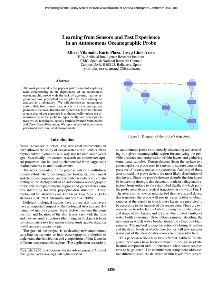
Figure 1: Diagram of the probe’s trajectory.
Introduction
Recent advances in optical and acoustical instrumentation
have allowed the study of ocean water constituents such as
phytoplankton dynamics in a way not feasible some years
ago. Specifically, the current research on underwater optical properties can be used to characterize from large scale
marine patterns to small scale events.
The work presented in this paper is part of a multidisciplinary effort where oceanographic biologists, mechanical
and electronic engineers, and computer scientists are collaborating in the deployment of an autonomous oceanographic
probe able to explore marine regions and gather water samples interesting for their phytoplankton structure. These
phytoplankton structures are known as Thin Layers (Dekshenieks et al. 2001; Stramska and Stramski 2005).
Different biological studies have proved that thin layers
have an important impact on the biological structure and dynamics of marine systems. Nevertheless, because the composition and location of the thin layers vary with the time
and they are small structures (their range in thickness is from
few centimeters to a few meters), their study and localization
is still an open research topic.
The goal of the project is to develop new autonomous
sampling instruments to help oceanographic biologists to
understand the distribution and composition of thin layers in
different oceanographic regions. The application scenario is
an autonomous probe continuously descending and ascending in a given oceanographic region for analyzing the possible presence and composition of thin layers and gathering
some water samples. During descent (from the surface to a
given depth) the probe uses its sensors to capture data on the
presence of organic matter in suspension. Analysis of these
data inboard the probe detects the most likely distribution of
thin layers. Since the probe’s descent disturbs the thin layers
by its passing through, this descent is made in a diagonal trajectory from surface to the established depth, at which point
the probe ascends in a vertical trajectory, as shown in Fig. 1.
The ascension is now on undisturbed thin layers, and during
this trajectory the probe will use its water bottles to obtain
samples at the depths in which these layers are predicted to
be according to the analysis of the sensor data. There are two
main issues to solve here: (1) determining the number, depth
and shape of thin layers, and (2) given the limited number of
water bottles (around 10) to obtain samples, deciding the
moments in which water bottles should be closed to obtain
samples. The method to map the action of closing N bottles
and the depth levels at which these bottles will take samples
is not part of the identification component presented here.
This paper describes how two different Artificial Intelligence techniques have been combined to design an identification component able to determine when water samples
have to be gathered. The identification component addresses
two different tasks: the detection of thin layers from several
c 2010, Association for the Advancement of Artificial
Copyright Intelligence (www.aaai.org). All rights reserved.
1859
algorithm to detect irradiance peaks. mPSO is an optimization technique based on the movements of a collection of
particles that are selectively sampling a complex function
landscape (Poli, Kennedy, and Blackwell 2007).
Moreover, each algae group has specific characteristics
that produce different irradiance responses. This diversity
of response requires a two-step approach, where first main
algae type has to be identified and only then the other parameters may be precisely determined. Thus, a wrong identification of the algae group may produce a higher error in
determining the other parameters. The current simulations
cover four different types of algae families.
We have designed a Case-Based Reasoning (CBR) module for the characterization of the thin layers. CBR is an AI
technology that directly reasons from previous experiences
(Leake 1996). In our domain this feature is interesting because the nature of the domain knowledge is empirical, and a
theoretical biological model is not yet available. Moreover,
because CBR is a technology where reasoning and learning are intimately connected, it facilitates future steps of the
project.
Figure 2: Diagram of the component’s architecture.
data streams (coming from inboard optical sensors continuously measuring); and the characterization of their composition and location. The first task is accomplished with a
swarm approach whereas the second task is performed by a
case-based reasoning module.
The paper is organized as follows: the next section describes the task performed by the AI component and details
the design of two different AI modules; then we empirically
evaluate the performance of the identification component
by using 300 simulated environments and, finally, we draw
some conclusions and discuss the future research lines.
The mPSO module
Particle Swarm Optimization (PSO) aims at producing a collaborative intelligent behavior based on the metaphor of social interaction (Kennedy and Eberhart 1995). The movements of each particle are based on combining a cognitive
model with a social model. The cognitive model drives each
particle to its best position so far. The social model drives
each particle to the best position found by particles in its
neighborhood.
In PSO, each particle has a position p~i and a velocity ~vi .
Initially, the set of particles is randomly distributed with a
random initial velocity in the search space, which is a 2dimensional matrix (depth × frequency). The position and
velocity of each particle is modified iteratively: after a particle moves, the sensor value associated to the current particle’s position is read. The two equations that govern the
movements of each particle are the following:
The identification component
The identification component addresses two different issues:
the detection of possible thin layers and the characterization of these thin layers. Regarding the first issue, spectral
downwelling irradiance distributions (Ed ) obtained by hyperspectral sensors are used to detect thin layers. From Ed ,
the following four parameters that characterize a thin layer
can be calculated: the main algae group, the thickness, the
concentration, and the depth. Specifically, concentration is
estimated by the attenuation coefficient Kd in a depth z for
a given wavelength λ as follows:
ln[Ed (z2 , λ)/Ed (z1 , λ)]
z2 − z1
(1)
~ (0, φ1 )(~bi − p~i ) + U
~ (0, φ2 )(~g − p~i )) (2)
~vi = χ(~vi + U
where z1 , z2 are the previous and subsequent depths to the
target z where Ed was measured.
Applying the previous formula we may determine the possible presence of thin layers by looking for irradiance peaks.
In the design of the identification component we used 300
simulations generated by the experts using the HydrolightEcolight 5.0 numerical model (Mobley and Sundman 2008).
Each simulation provides the measurements of the downwelling irradiance with a depth resolution of 5cm and a
spectral resolution of 1nm for a given marine scenario.
Specifically, we work with scenarios where two different
thin layers (varying in depth, thickness, and concentration)
are present.
Nevertheless, the sensors provide a huge amount of data,
and only a low consuming algorithm is feasible. Thus, we
decided to use a multi Particle Swarm Optimization (mPSO)
where χ is the constant multiplier that ensures the convergence; p~i is the current position of the particle i; ~vi is the
velocity of the particle i; ~bi the best position found by the
particle i; ~g the global best solution found by the particles;
~ (0, φi ) represents a vector of random numbers uniand U
formly distributed in [0, φi ].
Since 2001, when Eberhart and Shi proposed the original
PSO for solving dynamic optimization problems, different
authors have proposed extensions to the original PSO algorithm, such as resetting the particles position frequently
or using a multi-swarm model (Poli, Kennedy, and Blackwell 2007) for improving its adaptiveness in dynamic environments (Blackwell 2007). In our project we have used
a multi-swarm approach inspired on the mQSOE model
Kd (z, λ) = −
p~i = p~i + ~vi
1860
(3)
similar cases are retrieved (Retrieve process), and how the
retrieved cases are used to predict the solution of a new situation (Reuse process).
The inputs for the CBR component are the sensor data and
the output from mPSO. Preliminary experiments showed
that only using concentration peaks, as detected in the previous section, was not enough: we need to take into account
both peaks and contour. For this purpose, we determine the
Discrete Fourier Transform (DFT) (Agrawal, Faloutsos, and
Swami 1993) of the sensor data, and select the first 4 coefficients as a higher-level representation of the thin layer
contour.
Case definition: A case is represented as pair hP, Si
where P is a problem description and S a solution description. In the thin layers domain a problem description is a
tuple P = hf1 , f2 , f3 , f4 , Kd , ωi, where f1 , . . . , f4 are the
first 4 coefficients of the DFT applied to the sensor data, Kd
is the attenuation coefficient (estimating concentration), and
ω is the full width at half maximum1 of a normal distribution
(estimating thickness). A solution is described by a tuple
S = hα, θ, ηi, where the three parameters are the algae type
(α), the (real) thickness (θ) and the (real) concentration (η).
Thus, when a new problem is addressed by the CBR module, the problem’s sensor data is transformed to DFT and
the first 4 coefficients obtained define the new case hP 0 , S 0 i.
The outcome of the CBR module for a new problem P 0 is a
prediction of a new solution S 0 , namely algae type, thickness
and concentration of the thin layer described by P 0 .
Figure 3: The mPSO algorithm working in a noisy environment.
(Fernandez-Marquez and Arcos 2009). The multi-swarm
approach is appropriate in multi-modal problems (i.e. when
several peaks appear at the same time). However, simply
dividing a global swarm into a set of independent swarms
does not guarantee success. At least a new operator has to
be introduced: the exclusion operator.
Exclusion operator: The exclusion operator is introduced
to ensure that two sub-swarms are not exploiting the same
peak, i.e. to guarantee swarm diversity. Two sub-swarms
are considered to be close to each other when their attractors
(best solutions) are within an exclusion radius. When this
occurs, the sub-swarm with a lower solution is reinitialized
in the search space.
Retrieve: The Retrieve process of CBR estimates the similarity of the new problem with those present in the case
base, in our module using an Euclidean distance over the
f1 , . . . , f4 coefficients. Since a coefficient is a complex
number (fj = rj + icj ), the Euclidean distance is computed over 8 dimensions (r1 , . . . , r4 , c1 , . . . , c4 ). A number
k of more similar cases is the output of the Retrieve process.
Different experiments were performed to elucidate the value
of k, which was set (for the results reported here) to k = 3.
Launching swarms: Each time the probe completes a descendant path, the peaks detection algorithm is fired. The
peaks detection algorithm uses 4 swarms of 10 particles to
explore a given simulation (the measurements of a specific
marine scenario). The standard PSO parameters have been
set following (Blackwell 2007), while the swarm exclusion
radius was set following (Blackwell and Branke 2005). We
only allow the access to 104 measures (i.e. each particle performs only 250 movements). Figure 3 shows an example of
a multi swarm exploring a multi peak environment. Notice
that the irregularity in the environment is generated by the
presence of noise affecting the measurements.
The output of mPSO is a set of detected thin layers expressed as pairs composed of depth and Kd (estimated concentration).
Reuse: The Reuse process builds a local model based on
the nearest cases (the k retrieved cases) and applies it to predict the solution of the new case. Specifically, the Reuse has
to determine the solution tuple hα0 , θ0 , η 0 i (i.e. algae type,
thickness and concentration) of the new case based on the
solutions (i.e. tuples hα, θ, ηi) of the retrieved cases. Algae
type α is determined by majority vote of the algae types in
the retrieved cases.
In order to predict the numerical values of the (real) thickness (θ) and the (real) concentration (η) we cannot directly
use the estimation of the input data (Kd and ω respectively).
For that purpose, we use the case base a second time, now
The CBR module
Case-Based Reasoning (Kolodner 1993) is an AI approach
that capitalizes on previous problem-solving experiences
when solving new problems, retrieving similar past cases
and reusing their solutions to determine the predicted solution for a new problem; see (Mantaras et al. 2005) for an
overview on CBR. This section presents the CBR model of
the probe indentification of thin layers: we will define what
a case is in the domain of thin layers (Case definition), how
1
The full width at half maximum (FWHM) is an estimation of
the extent of a function such as duration of a pulse in a waveform.
Specifically, FWHM is the difference between the two extreme values of the independent variable at which the dependent variable is
equal to half of its maximum value. Assuming that thin layer concentration has a normal distribution, FWHM can be computed from
the standard deviation.
1861
Figure 4: Linear regression models (for each algae type) between estimated concentration (Kd ) and real concentration
(η).
Figure 5: Linear regression models (for each algae type) between estimated thickness (ω) and real thickness (θ).
a radiative transfer numerical model that computes spectral
radiance distributions and related quantities for water bodies. A scenario consists of measurements of the attenuation
coefficient (Kd ) from 0 to 15 meters depth (with a sample at
each 5cm) and ranging from 400nm to 650nm (with a spectral resolution of 1nm). Each scenario has two thin layers
at different depths (i.e. we have models of 600 thin layers).
The thin layers present in a simulation vary in depth (from
4m to 12m), thickness (from 0.4m to 1.4m), and concentration (from 4mg/m3 to 20mg/m3 ). Finally, we applied
different noise levels to the input signals in order to test the
robustness of our approach.
to determine how estimators Kd and ω diverge from the real
values θ and η in each of the known cases. Moreover, since
this divergence may depend on the algae type, we use a linear regression method to find the multiplicative factor that
relates estimated values to real values for each algae type.
Figure 4 shows the linear regression model relating estimated concentration (Kd ) with the real concentration (η) for
the 4 algae types (each one represented as a different line).
The predicted value for real concentration (η) is determined
using the linear regression model of algae type α at the value
Kd .
Similarly, Figure 5 shows the linear regression model relating estimated thickness (ω) with the real thickness (θ) for
the 4 algae types; the figure shows that the linear regression
model for thickness is much less dependent on algae type
than before. The predicted value for real thickness (θ) is determined using the linear regression model of algae type α
at the value ω.
In summary, the CBR module outputs the solution S 0 =
hα0 , θ0 , η 0 i for a problem P 0 by predicting the algae class
α0 of the most similar cases and predicting thickness θ0 and
concentration η 0 by a regression-based adaptation of the estimators of thickness and concentration in the input of the
current problem.
Thin layers detection
We used 40 particles grouped in 4 different swarms, i.e. each
swarm with 10 particles. Our method required accessing just
13% of the 7.5×10⁴ measurements existing for each model.
The results presented below are the average of 20 runs per
scenario.
Because each simulation contains two different thin layers, the difficulty of detecting both thin layers depends on
their proximity and on their size difference. A detailed analysis of the experiments revealed that the proximity factor
(with a minimum value of 3.5 meters) does not increase the
average error. On the other hand, the hardest problems are
those where the first thin layer presents a high concentration and the second layer presents a low concentration. In
these simulations some of the runs were not able to detect
the second thin layer (see 1st row in Table 1).
For the simulations where the thin layer is detected, the
2nd row in Table 1 shows the peak depth error in centimeters. First, notice that the level of error in thin layer detection is independent of the depth. Moreover, the experiments show that the error is smaller than the depth resolution
(5cm). Finally, the algorithm detection of thin layers’ depth
Experiments
The goal of the experiments was to validate the accuracy and
robustness of the identification component. Two different
sets of experiments were designed to test separately the peak
detection module and the case-based reasoning module.
For testing our system, we have used 300 water column
scenarios generated by the experts using the Hydrolight numerical model. Hydrolight (Mobley and Sundman 2008) is
1862
Noise
Failures
Error
Std.Dev.
0%
1.38
2.8
3.0
10 %
1.62
3.3
6.0
20 %
1.64
3.4
7.4
30 %
1.67
3.9
8.3
40 %
1.75
4.1
9.8
Algae Types
Precision
Sensitivity
Specificity
Accuracy
50 %
1.82
4.2
10.8
Table 1: Peak detection failures (%), error (cm), and standard deviation, given noise levels ranging from 0% to 50%.
A
0.97
0.93
0.99
0.97
B
0.96
0.96
0.98
0.98
C
0.95
0.94
0.98
0.97
D
0.93
0.98
0.97
0.98
Table 2: Algae identification analysis with a 30% of noise.
Algae Types
Concentration
Thickness
A
0.95
0.96
B
0.97
0.97
C
0.96
0.96
D
0.97
0.97
Table 3: Concentration and thickness accuracy on the 4 algae types.
phytoplanktonic thin layers given the input captured by the
oceanographic probe sensors. Our development uses two AI
techniques, namely Particle Swarm Optimization and CaseBased Reasoning. A major issue in developing a system that
works upon sensor data is to dramatically reduce the dimensionality of the problem. Sensor data of one problem is, in
our domain, a matrix with 75,000 elements, where every element is a floating point number. The mPSO module samples
about a 10% of the matrix data, already achieving a large
reduction. The mPSO output is a vector of radiance values
at 250 frequencies, achieving a second large dimensionality
reduction.
Since only using concentration peaks was not sufficient,
we needed to capture information about the contour of the
thin layers. The DFT operation effectively captures this information, and allows another large dimensionality reduction by selecting only the first 4 coefficients. The CBR module is then able to work with a highly compact and efficient
case representation, where the problem is described by 10
dimensions: the Fourier coefficients’ 4 complex numbers,
the attenuation coefficient, and the FWHM width.
Although our experiments are based on synthetic data, the
case-base and the sensor data are based on commercial simulators and have been generated by experts from the Marine
Technology Unit (UTM-CSIC). The experiments show that
the accuracy of the system is high, and thus we expect that
it would constitute an adequate identification module for the
probe when deployed in the second half of 2010. Notice that
the probe, by design, needs to have a robust decision system
from the start — engineering it from synthetic but reasonably accurate data was a necessity.
We plan to acquire real data from the deployment of the
oceanographic probe, on top of which we can apply the same
methodology and obtain a second, more adapted, decision
module for an autonomous probe. Undoubtedly real data
may present new challenges to address, but our current work
has shown the feasibility of using these or other AI techniques in this problem domain.
The final decision of when to take samples (i.e. closing
the water bottles in the probe) remains future work. These
decisions are a direct consequence of the number of bottles,
the number of detected thin layers, and the characterization
Figure 6: Accuracy in algae identification when applying
noise levels ranging from 0% to 50%.
is robust in the presence of noise, since both failure rate and
error are not degraded excessively with a noise up to 50%.
Characterizing thin layers
This subsection presents an experimental evaluation of thin
layers characterization performed by the CBR module. For
this purpose, as before, we strain the CBR module by applying noise levels ranging from 0% to 50%.
The first task of the CBR module is to identify the main
algae type in a thin layer. We asses the CBR module’s accuracy by a set of experiments performing 10-fold crossvalidation. Before applying noise to the data, Figure 6 shows
that accuracy is between 98% and 100% depending on the
algae type. Applying noise up to 30% the identification accuracy is not degraded significantly (see Figure 6). Notice
that the accuracy of algae type B is kept at 100% up to a
noise level of 20%. At noise levels higher than 30%, although the performance declines, accuracy is still around
95% at 50% of noise.
Table 2 summarizes the precision, sensitivity, and specificity of the CBR module with a noise level of 30% (the
noise cut level). Although there are differences on these
measures depending on the algae type, they are not statistically significant. Finally, Table 3 shows the accuracy of
the CBR module in predicting concentration and thickness
in the scenario without noise for the 4 algae types. Since the
error is less than 5%, the identification is robust enough for
an autonomous probe.
Conclusions and future work
We have presented the design and development of an autonomous system that determines the depth and features of
1863
Figure 7: Snapshot of the Simulator Framework.
of these thin layers in terms of algae type, depth, concentration and thickness. In our planned approach, the probe will
include a set of expert-defined rules that perform this mapping, implementing (1) default strategies (e.g. one sample
at each thin layer’s concentration peak) and (2) immersionspecific tactical decisions (e.g. the biologist may indicate
preference of information sampling for specific algae types).
Immersion-specific tactical decisions are needed to override
defaults, and ensure the capability of the probe to perform
repeated immersions in the same area and acquire several
different collections of samples. Ensuring this variety of
samples is critical for oceanographic probes.
ments, volume 51 of Studies in Computational Intelligence.
Springer. 29–49.
Dekshenieks, M.; Donaghey, P.; Sullivan, J.; Rines, J.; Osborn, T.; and Twardowski, M. 2001. Temporal and spatial
occurrence of thin phytoplankton layers in relation to physical processes. Marine Ecology Progress Series 223:61–71.
Fernandez-Marquez, J., and Arcos, J. 2009. An evaporation
mechanism for dynamic and noisy multimodal optimization.
In Proceedings of the 10th Genetic and Evolutionary Computation Conference (GECCO’09), 17–24.
Kennedy, J., and Eberhart, R. C. 1995. Particle swarm optimization. In Proc. of the IEEE international conference on
neural networks IV, 1942–1948.
Kolodner, J. 1993. Case-based Reasoning. Morgan Kaufmann.
Leake, D. B., ed. 1996. Case-Based Reasoning: Experiences, Lessons and Future Directions. MIT Press.
Mantaras, R.; McSherry, D.; Bridge, D.; Leake, D.; Smyth,
B.; Craw, S.; Faltings, B.; Maher, M.; Cox, M.; Forbus, K.;
Keane, M.; Aamodt, A.; and Watson, I. 2005. Retrieval,
reuse, revision, and retention in CBR. Knowledge Engineering Review 20(3):215–240.
Mobley, C. D., and Sundman, L. K. 2008. Hydrolightecolight 5.0 user’s guide. Technical report, Sequoia Scientific, Inc., Bellevue, WA.
Poli, R.; Kennedy, J.; and Blackwell, T. 2007. Particle
swarm optimization. an overview. Swarm Intelligence 1:33–
57.
Stramska, M., and Stramski, D. 2005. Effects of a nonuniform vertical profile of chlorophyll concentration on remotesensing reflectance of the ocean. Applied Optics 44:1735–
1747.
Acknowledgments
The authors thank reviewers that helped to improve and correct this paper. The authors also want to thank Jaume Piera,
Elena Torrecilla, and Sergi Pons that designed and generated
probe scenarios. This work was partially funded by projects
ANERIS (CSIC-PIF08-15-2), Next-CBR (TIN2009-13692C03-01), and by the Generalitat de Catalunya under the
grant 2009-SGR-1434.
References
Agrawal, R.; Faloutsos, C.; and Swami, A. 1993. Efficient
similarity search in sequence databases. In Foundations of
Data Organization and Algorithms, volume 730 of Lecture
Notes in Computer Science. Springer Verlag. 69–84.
Blackwell, T., and Branke, J. 2005. Multiswarm, exclusion, and anti-convergence in dynamic environments. IEEE
Trans. Evolutionary Computation 10(4):459–472.
Blackwell, T. 2007. Particle swarm optimization in dynamic
environments. In Yang, S.; Ong, Y.-S.; and Jin, Y., eds., Evolutionary Computation in Dynamic and Uncertain Environ-
1864
