Proceedings of the Thirtieth AAAI Conference on Artificial Intelligence (AAAI-16)
Weighted A∗ Algorithms for Unsupervised Feature Selection
with Provable Bounds on Suboptimality
Hiromasa Arai, Ke Xu, Crystal Maung, Haim Schweitzer
{Hiromasa.Arai, ke.xu}@utdallas.edu Crystal.Maung@gmail.com, hschweitzer@utdallas.edu
Department of Computer Science, University of Texas (Dallas)
800 W Campbell Road, Richardson, TX 75080
Abstract
Identifying a small number of features that can represent the
data is believed to be NP-hard. Previous approaches exploit
algebraic structure and use randomization. We propose an algorithm based on ideas similar to the Weighted A* algorithm
in heuristic search. Our experiments show this new algorithm
to be more accurate than the current state of the art.
1
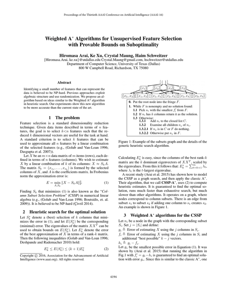
0. Put the root node into the fringe F .
1. While F is nonempty and no solution found:
1.1 Pick ni with the smallest fi from F .
1.2 If ni has k columns return it as the solution.
1.3 Otherwise:
1.3.1 Add ni to the closed list C.
1.3.2 Examine all children nj of ni .
1.3.2.1 If nj is in C or F do nothing.
1.3.2.2 Otherwise put nj in F .
The problem
Feature selection is a standard dimensionality reduction
technique. Given data items described in terms of n features, the goal is to select k<n features such that the reduced k dimensional vectors are useful for the task at hand.
A standard criterion is to select k features that can be
used to approximate all n features by a linear combination
of the selected features (e.g., (Golub and Van-Loan 1996;
Dasgupta et al. 2007)).
Let X be an m×n data matrix of m items (rows), each defined in terms of n features (columns). We wish to estimate
X by a linear combination of k of its columns: X ≈ Sk A.
The matrix Sk = (xs1 , . . . , xsk ) is formed by the selected
columns of X, and A is the coefficients matrix. In Frobenius
norm the approximation error is:
E = min X − Sk A2F
A,Sk
Figure 1: Example of the subsets graph and the details of the
generic heuristic search algorithm.
Calculating Ek∗ is easy, since the columns of the best rank-k
matrix are the k dominant eigenvectors of XX T
, scaled by
m
the eigenvalues. From this it follows that: Ek∗ = t=k+1 λt ,
where λt is the t-largest eigenvalue.
A recent study (Arai et al. 2015) has shown how to model
the CSSP as a graph search, and then apply the classic A∗ .
Their algorithm, that we call CSSP-A∗ , uses (2) to compute
heuristic estimates. It is guaranteed to find the optimal solution, runs much faster than exhaustive search, but much
slower than other algorithms. It operates on a graph, where
nodes correspond to column subsets. There is an edge from
subset s1 to subset s2 if adding one column to s1 creates s2 .
An example is shown in Figure 1.
(1)
Finding Sk that minimizes (1) is also known as the “Column Subset Selection Problem” (CSSP) in numerical linear
algebra (e.g., (Golub and Van-Loan 1996; Boutsidis, et. al.
2009)). It is believed to be NP-hard (Çivril 2014).
2
Heuristic search for the optimal solution
3
Sk∗
Let
denote a (best) selection of k columns that minimizes the error in (1), and let E(Sk∗ ) be the corresponding
(minimal) error. The eigenvalues of the matrix XX T can be
used to obtain bounds on E(Sk∗ ). Let Ek∗ denote the error
of the best approximation of X in terms of a rank-k matrix.
Then the following inequalities (Golub and Van-Loan 1996;
Deshpande and Rademacher 2010) hold:
Ek∗ ≤ E(Sk∗ ) ≤ (k + 1)Ek∗
Weighted A∗ algorithms for the CSSP
Let ni be a node in the graph with the corresponding subset
Si . Set j = |Si | and define:
gi Error of estimating X using the j columns in Si .
fi Error of estimating X using the j columns in Si and
additional “best possible” k − j vectors.
hi g i − fi .
Let g∗ be the smallest possible error in Equation (1). It was
shown by (Arai et al. 2015) that running the algorithm in
Fig.1 with fi = gi −hi is guaranteed to find an optimal solution with error g∗ . Since this is similar to the classic A∗ , one
(2)
c 2016, Association for the Advancement of Artificial
Copyright Intelligence (www.aaai.org). All rights reserved.
4194
fi
gi − hi + gi
gi − hi + hi
gi − hi + bi
Name
CSSP-WA*-g
CSSP-WA*-h
CSSP-WA*-b
k
20
60
100
Suboptimality Bound
g∗ ≤ g∗ + g0
g∗ ≤ g∗ + h0
g∗ ≤ (1 + (k + 1))g∗
k
3
4
5
may expect an improved run time by the classic Weighted
A∗ algorithm , which replaces hi with (1+)hi (Pearl 1984).
Unfortunately we have found experimentally that the resulting algorithm runs even slower than the CSSP-A∗ . However, we discovered that assigning weights differently produces the desired improved runtime, with precise bounds on
suboptimality. Specifically, we propose to use the following
heuristic for a Weighted A∗ algorithm for the CSSP:
A*
{6, 84, 121}
{6, 84, 121, 329}
{6, 84, 121, 329, 5376}
WA*-b
{6, 84, 121}
{6, 84, 121, 329}
{6, 84, 121, 329, 5376}
comparison on the TechTC01 dataset of size (163×29,261).
The results of the CSSP-WA* variants were compared to
the following two algorithms: 1. The GKS, considered one
of the best among the pure algebraic algorithms (Golub and
Van-Loan 1996). 2. The randomized two-stage-method that
we call LEV GE (Boutsidis, et. al. 2009). It is considered
one of the top randomized algorithms. The results are shown
in figures 3,4. Observe that the CSSP-WA*-b always come
as best in Figure 3. In Figure 4, observe that the CSSP-WA*
found the optimal solution in each case. (The CSSP-WA*g and the CSSP-WA*-h also find the optimal solution in
this case.) Observed that the CSSP-WA* variants were much
faster than the CSSP-A*.
with ≥ 0, vi ≥ 0. We call such an algorithm a CSSP-WA∗ .
Suboptimality
Let n∗ be an optimal solution node, and let g∗ be the corresponding (optimal) error value. Suppose vi ≥ 0 can be
computed at each node, and fi =gi −hi +vi .
Theorem 1: If fi is used by the algorithm in Figure 1, it will
terminate with a solution satisfying: g∗ ≤ g∗ + vmax , where
vmax = maxi vi . See (Arai et al. 2016) for the proof.
The theorem is useful for proving bounds on suboptimality, but by itself it does not provide guidance as to what constitutes a useful vi . The following corollary suggests that vi
should be chosen monotonically decreasing along any path.
Under this condition the bound becomes tighter during the
run of the algorithm.
Corollary 1: Let g∗ , g∗ , vi be as above. Suppose vi is monotonically decreasing along any path. Let nr be a visited node
in the path to the solution, and let vr be the value computed
at nr . Then: g∗ ≤ g∗ + vr . (Proof: Apply Theorem-1 to the
subgraph rooted at nr .)
We note that the guarantee in the corollary may be much
stronger than the guarantee provided by the theorem since
vr may be much smaller than v0 , the value of vi at the root.
Three choices for vi are shown in Figure 2: gi , hi , and bi .
The function bi is computed in a similar way to the upper
bound in (2) and gives multiplicative bounds on suboptimality (see (Arai et al. 2016) for details). It can be shown that
the functions gi , hi produce the same algorithm with different range values of .
5
Concluding remarks
The unsupervised feature selection problem that we consider, the CSSP, is a practical problem that was heavily studied for over 50 years. Our solution, using ideas from heuristic search, is more accurate than all currently available practical approaches. This comes at the expense of a longer running time. Still, our approach should be a preferred choice
when an increase in running time can be tolerated.
References
Arai, H.; Maung, C.; and Schweitzer, H. 2015. Optimal
column subset selection by A-Star search. In AAAI’15, 1079–
1085.
Arai, H.; Maung, C.; Xu K.; and Schweitzer, H. 2016. Unsupervised feature selection by heuristic search with provable
bounds on suboptimality. In AAAI’16.
Boutsidis, C.; Mahoney, M. W.; and Drineas, P. 2009. An
improved approximation algorithm for the column subset selection problem. In SODA’09, 968–977.
Çivril, A. 2014. Column subset selection problem is ughard. Journal of Computer and System Sciences 80(4):849–859.
Dasgupta et al. 2007. Feature selection methods for text
classification. In KDD’07, 230–239.
Deshpande, A., and Rademacher, L. 2010. Efficient volume
sampling for row/column subset selection. In FOCS’10, 329–
338.
Golub, G. H., and Van-Loan, C. F. 1996. Matrix computations.
Pearl, J. 1984. Heuristics. Addison-Wesley.
Computing the heuristics
In calculating fi , gi , hi we follow (Arai et al. 2015). Let
Si be the columns at node ni , and set j = |Si |. Compute the matrix Qi , an orthogonal basis to Si . Compute:
Xi = X − Qi QTi X, and Bi = Xi XiT .
Let λ1 ≥ . . . ≥ λm
m
be the eigenvalues of Bi . Then: gi = t=1 λt = Xi 2F ,
j
m
hi = t=1 λt , fi = t=j+1 λt .
4
WA*-b/(time)
6.9E+05/(0.80)
1.3E+05/(5.68)
2.1E+04/(14.47)
Figure 4: Column indices selected by A∗ and WA∗ -b(=0.5)
fi = gi − hi + vi
3.2
LEV GE/(time)
8.7E+05/(0.67)
1.7E+05/(1.93)
2.8E+04/(3.15)
Figure 3: Error and time(min) comparison(WA* uses =0.5.)
Figure 2: Three CSSP-WA* algorithms
3.1
GKS/(time)
7.1E+05/(0.02)
1.5E+05/(0.04)
2.8E+04/(0.06)
Experimental results
We tested and compared our algorithms to the state of the
art and the CSSP-A∗ on several datasets. We describe here a
4195