Proceedings of the Twenty-Fifth Innovative Applications of Artificial Intelligence Conference
Case-Based Meta-Prediction for Bioinformatics
Xi Yun1, Susan L. Epstein1, 2, Weiwei Han3, and Lei Xie1, 2
Department of Computer Science
The Graduate Center and 2Hunter College of The City University of New York
New York, NY 10065 USA
3
Key Laboratory for Molecular Enzymology and Engineering of Ministry of Education,
Jilin University, Changchun 130023, P. R. China
xyun@gc.cuny.edu, susan.epstein@hunter.cuny.edu, weiweihan@jlu.edu.cn, lei.xie@hunter.cuny.edu
1
A meta-predictor combines individual predictors to
evaluate possibilities. Conventional bioinformatics metapredictors use consensus scoring, which averages scores on
the new example from an ensemble of individual predictors
or takes a majority vote among them (Charifson et al.,
1999; Clark et al., 2002). Although consensus scoring
seeks reliability, it ignores similarities between examples,
as well as domain-specific and example-specific information about individual predictors. As a result, if most
predictors are inaccurate on an example, consensus scoring
is too, even if some predictor is highly reliable there. In
contrast, CBMP gauges its ensemble of predictors on a feature-based set of cases similar to the new example.
CBMP was originally developed to expedite search on
constraint satisfaction problems. The domain of investigation here, however, is prediction of protein-ligand interaction, an important but unsolved problem in bioinformatics
(Huang and Zou, 2010). To the best of our knowledge, this
is the first work that exploits case-based reasoning to combine multiple protein-ligand docking programs.
This paper makes two major contributions. First, it
demonstrates that case-based reasoning improves the predictive accuracy of protein-ligand interaction on different
receptors. This indicates its potential support for a broad
range of bioinformatics applications. Second, it introduces
a method to estimate the reliability of case-based prediction. Although the ability to report such reliability is essential for computational prediction in biological experiments,
it is rarely available from bioinformatics methods.
The next section of this paper introduces relevant back-
Abstract
Before laboratory testing, bioinformatics problems often require a machine-learned predictor to identify the most likely
choices among a wealth of possibilities. Researchers may
advocate different predictors for the same problem, none of
which is best in all situations. This paper introduces a casebased meta-predictor that combines a set of elaborate, preexisting predictors to improve their accuracy on a difficult
and important problem: protein-ligand docking. The method
focuses on the reliability of its component predictors, and
has broad potential applications in biology and chemistry.
Despite noisy and biased input, the method outperforms its
individual components on benchmark data. It provides a
promising solution for the performance improvement of
compound virtual screening, which would thereby reduce
the time and cost of drug discovery.
Introduction
The wealth of possibilities to investigate during search often requires a predictor, an algorithm that identifies the
most likely value or class for an example. Although many
such predictors exist, typically no single one consistently
outperforms all the others on a large, diverse set of benchmark examples. This issue is particularly serious in bioinformatics, where data is often noisy and biased. The thesis
of this paper is that the close predictive accuracy of a single predictor on similar examples supports reasoning from
a set of predictors about a new example. This paper introduces an approach based on case-based reasoning: CBMP
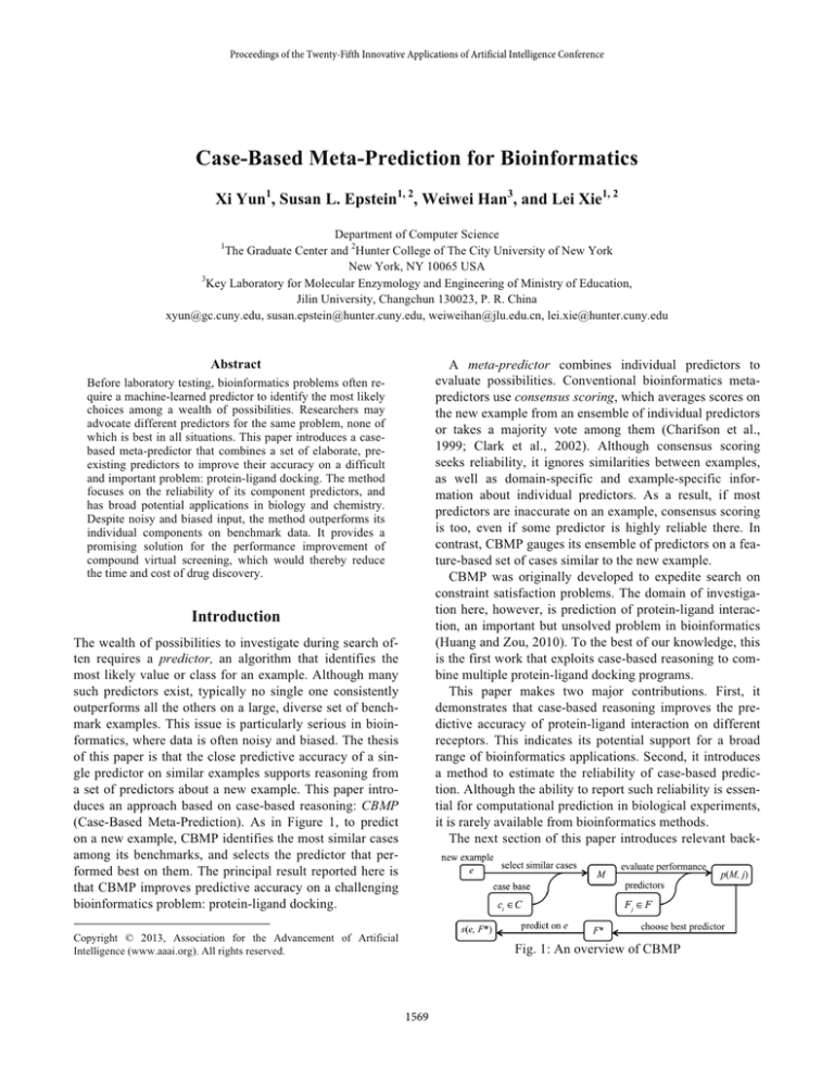
(Case-Based Meta-Prediction). As in Figure 1, to predict
on a new example, CBMP identifies the most similar cases
among its benchmarks, and selects the predictor that performed best on them. The principal result reported here is
that CBMP improves predictive accuracy on a challenging
bioinformatics problem: protein-ligand docking.
Copyright © 2013, Association for the Advancement of Artificial
Intelligence (www.aaai.org). All rights reserved.
Fig. 1: An overview of CBMP
1569
Our new method, CBMP, was inspired by our earlier
work on parallel scheduling of constraint satisfaction solvers on a new problem, based on their performance on a set
of similar problems (Yun and Epstein, 2012). Both constraint satisfaction and PLD face similar challenges under
this approach. They must identify a representative set of
similar instances, and they require refined representations
for cases and accurate similarity metrics for pairs of cases.
CBMP extends CBR and PLD prediction in several
ways. First, it executes extensive offline computation to
calculate case descriptions, whose features may differ from
those on which the individual predictors rely. In particular,
while the individual PLD predictors that CBMP references
here all address three-dimensional chemical conformation,
CBMP itself gauges case similarity from physiochemical
and topological properties derived from two-dimensional
chemical structure. The premise is that similar ligands are
likely to bind to a protein in a similar way. CBMP also
proposes a reliable predictor performance metric, and integrates similarity-based reference-case selection with performance-based predictor selection into a single framework. Finally, CBMP can report its confidence in its prediction, and has greater accuracy on confident cases.
The work reported here takes three PLD tools as scoring
functions: eHiTS1, AutoDock Vina2, and AutoDock3. Each
has its own strategies for conformational sampling and for
scoring. Both AutoDock and AutoDock Vina use a genetic
algorithm to search the ligand conformational space. In
contrast, eHiTS uses a fragment-based systematic search to
sample the conformational space of ligands. AutoDock’s
scoring function applies a force-field-based approach derived from physical phenomena. AutoDock Vina’s empirical scoring functions sum individual energy terms (e.g.,
Van der Waals, electrostatic), and then train parameters on
co-crystallized protein-ligand complexes with experimentally determined binding affinities. Finally, eHiTS combines empirical and knowledge-based scores trained from
known protein-ligand complexes. Because of their different algorithms and training data, these methods often have
dramatically different performance on the same data set.
No single method consistently outperforms the others.
ground on protein-ligand docking and case-based reasoning. Subsequent sections describe CBMP, evaluate its performance on different receptors, and discuss the results.
Background and Related Work
A ligand is a small molecule that can bind to a specific position (often an open cavity) in a protein. Protein-ligand interaction is the basis of many biological processes, and the
central topic of rational drug design. Computational tools
are critical to understanding molecular mechanisms such as
protein-ligand interaction. These tools seek to reduce the
time and cost required by laboratory experiments that
search for a ligand for a receptor (Huang and Zou, 2010).
Protein-ligand docking (PLD) is a molecular modeling
technique that evaluates a ligand’s orientations and conformations (three-dimensional coordinates) when it is
bound to a protein receptor or enzyme. For drug discovery,
PLD supports virtual high-throughput screening (VHTS) on
large libraries of available chemicals. Thousands of compounds may be tested in a single docking run (Morris et al.,
1998; Trott and Olson, 2010; Zsoldos et al., 2006). Many
PLD programs explore the search space of possible orientations and conformations to identify those with the strongest (i.e., minimal) total binding energy in a protein-ligand
complex. Binding energy prediction thus is critical for
PLD, but most PLD software does it poorly.
As a result, considerable effort has been devoted to the
combination of multiple scoring functions for more reliable
evaluation (Wang and Wang, 2001). These methods either
average scores or take the majority opinion from a set of
algorithms that predict the strength with which a protein
will bind with a ligand. The success of typical consensus
strategies in VHTS is marginal, as shown in our results.
Novel consensus scoring methods have been proposed
for VHTS. A multistep procedure chained multiple virtual
ligand-screening programs, and studied the impact on
speed and accuracy (Miteva et al., 2005). A bootstrapbased consensus scoring method improved the performance of a single PLD scoring function (Fukunishi et al.,
2008). That approach exploited ensemble learning to combine multiple scores from predictors that used the same
function but different energy-parameter sets. None of these
methods, however, combines output from different PDL
programs based on similarities between examples and on
example-specific information about individual predictors.
CBMP addresses the PLD challenge in VHTS with a
meta-prediction method based on case-based reasoning
(CBR). CBR is a problem-solving paradigm that retrieves
and uses knowledge about previously experienced examples (cases) to solve a new problem. A recent CBR system,
for example, diagnosed a patient based on diagnoses for
the most similar previous patients (Pous et al., 2009).
Case-based Scoring with CBMP
Each example here is a chemical compound, represented
for CBMP by its fingerprint, a boolean feature vector that
reports the presence or absence of chemical properties
(e.g., whether it is a hydrogen-bond donor, or its topological distance between two atoms lies in some range). This
1
http://www.simbiosys.ca/ehits/ehits_overview.html
http://vina.scripps.edu/
3
http://autodock.scripps.edu/
2
1570
examples drawn from DUD (Directory of Useful Decoys),
a set of benchmarks for virtual screening (Huang et al.,
2006). A decoy is a molecule that is similar to a ligand in
its physical properties but dissimilar in its topology. Along
with each ligand, DUD includes 36 decoys intended to
challenge a PLD algorithm. A good scoring algorithm
should predict low binding-energy scores (for molecular
stability) on real ligands, but high binding-energy scores
for decoys.
Typically, different PLD scoring functions predict on incomparable scales, a concern for a meta-predictor that relies upon multiple scoring functions. We therefore use a
simple but robust rank-regression scoring mechanism that
uniformly maps the raw scores from any Fj ∈ F to a normalized rank score. The scores from Fj thereby become independent of its scale; they reflect only the preference of Fj
for one case over another. More formally, given a set C of
n reference cases, CBMP calculates rank-regression scores
as follows. For each Fj ∈ F, CBMP sorts the s(i,j) raw
scores for ci ∈ C in ascending order, replaces the scores
with their rank, and then normalizes that rank in [0,1].
Note that this process assigns smaller scores to higherranked cases, to coincide with the premise that a smaller
binding-energy score is better.
Intuitively, a scoring function that accurately distinguishes ligand set L from decoy set D in set C (where
D ∪ L = C) should predict lower scores for ligands and
higher scores for decoys. In other words, scoring function
Fj is more accurate on ligand l only if its prediction for l is
generally lower than its predictions for D. Similarly, Fj is
more accurate on decoy d only if its prediction for d is
generally higher than its predictions for L. In summary, the
accuracy of the algorithm Fj on example ci is
Algorithm 1: CBMP (e, F, C, d)
(1) Select cases M ⊆ C most similar to e under d.
(2) Calculate s(e,j) for all Fj ∈ F.
(3) Combine s(e, j) for all Fj ∈ F to predict a score for e.
fingerprint includes hundreds of features whose values are
readily calculated from such software as openbabel4.
Let e be a new example for prediction, C the set of previously experienced, stored cases, and N(c) the number of
1’s in c ∈ C. The similarity metric between an example e
and a case ci ∈ C is defined by the Tanimoto coefficient:
d(e, ci) = N(e & ci) / N(e | ci )
(1)
This is the ratio of the number of features present in their
intersection to the number of features present in their union.
Let F be a set of scoring functions, where each scoring
function Fj ∈ F predicts score s(i, j) on case ci, and let p(i, j)
denote the predictive accuracy of Fj on ci. CBMP, our
case-based meta-predictor for example e, case set C, metric
d, and scoring functions F, appears in Algorithm 1.
Step 1 in Algorithm 1 assembles M, a set of cases most
similar cases to e. In step 2, each scoring function Fj predicts a score for e based on Fj’s predictions on M. Intuitively, experience from a case closer to the new example e
should provide a more reliable prediction for e. Here,
therefore, the prediction of Fj for e is calculated as a linear
combination of Fj’s scores for all the cases in M:
(2)
s e, j = ∑ wi s(i, j)
( )
ci ∈M
where weight wi quantifies the similarity between e and ci.
Here wi is from equation (1), but another d or computation
of from properties of e alone would be an alternative.
Step 3 in Algorithm 1 combines the scores from all Fj in
F on the cases in M to make a final prediction for e. Intuitively, a prediction from a scoring function that performs
better on M should have more influence on the final prediction. Let p(M, j) denote a set-based performance measurement for the overall predictive accuracy of Fj on the cases
in M. Rather than treat all cases in M equally, CBMP emphasizes cases more similar to e, again with weight wi:
(3)
p(M, j) = ∑
w p (i, j )
ci ∈M
⎧ {c ∈ D | s(c , j) > s(c , j)}
k
k
i
⎪
{ck ∈ D}
⎪
p(i, j) = ⎨
⎪ {ck ∈ L | s(ck , j) < s(ci , j)}
⎪
{ck ∈ L}
⎩
(6)
if ci ∈ D
The performance score produced by equation (6) lies in
[0,1]. The higher its value, the better the performance.
i
There are several possible ways to combine the s(e,j)
scores based on multiple predictions p(M, j). Here we use a
winner-take-all approach, applicable to both discrete and
continuous values. We identify F*, the Fj ∈ F that performs best on M, and report its score on e:
(4)
s(e, F * ) = s(e, argmax j p(M, j))
Empirical Design
Each of our experiments has a predictor predict the score
(i.e., binding energy) of a chemical e to a receptor. We examine the predictive accuracy of five predictors: three individual predictors (eHiTS, AutoDock Vina, AutoDock)
and two meta-predictors. The meta-predictors are CBMP,
where F is those three individual predictors, and RankSum,
a consensus scoring method described below.
Each predictor was applied to two receptors from DUD:
gpb and pdg. All three individual predictors perform relatively poorly on them, and one, eHiTS, is the worst of the
Application to Protein-Ligand Docking
This section tests CBMP on protein-ligand docking with
4
if ci ∈ L
http://openbabel.org/wiki/Main_Page
1571
|M| cases in C most similar to e, and used equation (6) to
evaluate the accuracy of each predictor across all cases in
M. CBMP then chose the individual predictor with the best
predictive accuracy on M, and reported as a score the rankregression score on e from that best individual predictor.
three on one but the best on the other. Both receptors therefore together challenge CBMP to choose the individual
predictor that will perform best on each chemical.
First, each individual predictor Fj calculated scores s(i,j)
for each of the ligands and decoys DUD provides. All three
individual predictors almost always returned a score. We
eliminated the very few without three scores; this left
n = 1901 chemicals for gpb, and n = 5760 for pdg. We
then replaced those scores with rank-regression scores, as
described in the previous section.
All experiments ran on an 8 GB Mac Pro with a 2.93
GHz Quad-Core Intel Xeon processor. We compare predictor performance on n chemicals with ROC (Receiver Operating Characteristic) analysis, using the R package ROCR.
The ROC curves illustrate the tradeoff between true positive and false positive rates, and thereby make explicit a
predictor’s hit ratio, an important factor in the decision to
actually test a likely ligand. (Classification accuracy alone
would be less beneficial, because the prevalence of decoys
biases the data sets. Simple prediction of every chemical as
a decoy would be highly accurate but target no chemicals
as worthy of laboratory investigation.)
RankSum is a typical bioinformatics meta-predictor.
Each individual predictor ranks chemicals with respect to
their rank-regression score. To predict the score on example e, RankSum then totals the ranks from the three predictors, where a lower score is better. Note that RankSum requires knowledge of the scores for all chemicals.
For CBMP, we first computed the similarities between
all nC2 pairs of chemicals, and recorded the five chemicals
most similar to each chemical, with their scores. We evaluated the three individual predictors with leave-one-out validation, as follows. In turn, each of the n chemicals for a
receptor served as the testing example e, while the other
n-1 served as the training cases in C. CBMP calculated the
Results and Discussion
We report first on a simple but effective version of Algorithm 1, where M is only a single case c, the one most similar to e. Thus, to predict a score for e, CBMP need only
compute p(c, j) for each Fj ∈ F. For |M| = 1, the ROC
curves in Figures 2 and 3 compare the performance of all
five predictors on receptors gpb and pdg, respectively,
based on the predictors’ scores and DUD’s class labels.
CBMP clearly outperforms the other predictors on both
receptors. In particular, CBMP outperforms the best individual predictor eHiTS on pdg, even though the majority
of its individual predictors perform poorly. In contrast, the
performance of RankSum on pdg was considerably worse,
because it requires accurate rankings from most of its constituent predictors for satisfactory performance, rankings
the individual predictors could not provide. We believe
that reliance on similar cases makes CBMP more resilient
than consensus scoring to occasional poor predictions from
individual predictors. (Of course, were all of F consistently
poor on all examples, CBMP would not succeed, but we
assume that the individual predictors were proved successful to some degree by other researchers.)
Confidence Analysis
0.0
0.2
0.4
0.6
0.8
0.6
0.8
CBMP
eHiTS
Vina
RankSum
Autodock
0.0
0.2
0.4
True positive rate
0.6
0.4
0.2
CBMP
eHiTS
Vina
RankSum
Autodock
0.0
True positive rate
0.8
1.0
1.0
In practice, CBMP should vary its confidence about its
predictions from one chemical to the next. For example, a
chemical may have a set M of closest neighbors that are actually relatively far from it (indicated by small similarity
1.0
0.0
False positive rate
0.2
0.4
0.6
0.8
1.0
False positive rate
Fig. 2: ROC curves for five PLD predictors on gpb.
Fig. 3: ROC curves for five PLD predictors on pdg.
1572
1.0
0.6
0.4
True positive rate
0.8
1.0
0.8
0.6
0.4
high
normal
low
0.0
0.2
True positive rate
0.0
0.2
high
normal
low
0.0
0.2
0.4
0.6
0.8
1.0
0.0
False positive rate
0.2
0.4
0.6
0.8
1.0
False positive rate
Fig. 5: ROC curves for confidence analysis on pdg.
values). As another example, a chemical may have a
neighbor on which individual scoring functions perform
poorly. In both situations, CBMP should be less confident
about its prediction. Intuitively, if CBMP can categorize
individual cases into different levels of confidence, it
might improve its performance on the cases where its confidence level is high.
Our confidence analysis considers three kinds of predictions, based on chemical similarity and scoring function
accuracy on M. Two chemicals are termed similar if and
only if their similarity is greater than t1 (here, 0.8), and dissimilar otherwise. A reliable predictor is one whose performance, as calculated by equation (6), is greater than t2
(here, 0.9); otherwise it is unreliable. Together t1 and t2 define three categories of predictive ability for scoring function Fj to predict on testing example e. A prediction has
high confidence if e’s closest neighbor c is similar to e and
Fj is reliable on c. A prediction has low confidence if c is
dissimilar to e and Fj is unreliable on c. In all other situations cases, a prediction has normal confidence.
Figures 4 and 5 isolate the performance of CBMP on
these three confidence levels for gpb and pdg, respective-
ly. For gpb, 31.93%, 47.76%, and 20.31% of the chemicals had high, normal, and low confidence, respectively.
For pdg, these percentages were 19.41%, 60.89%, and
19.70%. As expected, CBMP performed far better on the
high-confidence chemicals for both receptors than it did on
the full set. The benefit introduced by the confidence-based
classification for pdg is particularly promising: although
most candidate scoring functions had unreliable performance, confidence-based CBMP achieved almost perfect
prediction on the high-confidence chemicals.
CBMP assumes that a predictor’s accuracy on similar
chemicals will also be similar. To investigate whether twodimensional chemical similarity alone could predict ligands accurately, we ranked by similarity all pairs of possible chemicals that included at least one ligand for each receptor. A pair of two ligands was a match; otherwise, a
pair was a non-match. Ideally, match pairs should have
higher similarity scores than non-match pairs. Figure 6
shows the ROC curve for each receptor, based on the similarity scores and whether or not the pair was a match. Although chemical similarity alone clearly distinguishes ligands from decoys in the DUD benchmark data set, it provides very few likely ligands. CBMP’s predictive performance is considerably better than that, especially when
CBMP’s confidence is high.
0.6
Prediction from Larger Similarity Sets
0.4
Thus far, we have restricted the size of the similarity set M
to 1. Next we consider the impact of larger |M| on CBMP’s
performance. This time, each scoring function predicts for
e with equation (2), and evaluates its performance on M
with equation (3). CBMP then used the winner-take-all
policy from equation (4) to combine the predicted scores
from all three individual predictors. This allows CBMP to
consider the overall weighted performance of each predictor on a set of similar cases, and to formulate a weighted
prediction from the predictor with the best overall performance on those similar cases. Figures 7 and 8 show a clear
gpb
pdg
0.0
0.2
True positive rate
0.8
1.0
Fig. 4: ROC curves for confidence analysis on gpb.
0.0
0.2
0.4
0.6
0.8
1.0
False positive rate
Fig. 6: ROC curves for gpb and pdg based on computed
similarity and match/non-match labels of chemical pairs.
The marks at lower left correspond to the predictions based
only on the minimum chemical similarity score t1 = 0.8.
1573
Fig. 7 ROC curves for CBMP with different |M| on gpb.
Fig. 8 ROC curves for CBMP with different |M| on pdg.
performance improvement for |M| = 2 on both receptors.
For |M| = 3, however, this improvement is at best marginal.
Future work will investigate further the impact of the characteristics of the sample space C on CBMP’s performance.
rates from docking databases of three-dimensional structures into
proteins. J. Med. Chem. 42: 5100-5109.
Clark, R. D., A. Strizhev, J. M. Leonard, J. F. Blake and J. B.
Matthew 2002. Consensus scoring for Ligand/Protein
Interactions. J. Mol. Graphics Modell. 20: 281-295.
Fukunishi, H., R. Teramoto, T. Takada and J. Shimada 2008.
Bootstrap-based consensus scoring method for protein-ligand
docking. J. Chem. Inf. Model. 48(5): 988-996.
Huang, N., B. K. Shoichet and J. J. Irwin 2006. Benchmarking
Sets for Molecular Docking. J. Med. Chem. 49(23): 6789–6801.
Huang, S.-Y. and X. Zou 2010. Advances and Challenges in
Protein-Ligand Docking. Int. J. Mol. Sci. 11: 3016-3034.
Miteva, M. A., W. H. Lee, M. O. Montes and B. O. Villoutreix
2005. Fast Structure-Based Virtual Ligand Screening Combining
FRED, DOCK, and Surflex. J. Med. Chem. 48: 6012-6022.
Morris, G. M., D. S. Goodsell, R. S. Halliday, R. Huey, W. E.
Hart, R. K. Belew and A. J. Olson 1998. Automated Docking
Using a Lamarckian Genetic Algorithm and Empirical Binding
Free Energy Function. J. Comput. Chem. 19: 1639-1662.
Pous, C., D. Caballero and B. Lopez 2009. Diagnosing patients
with a combination of principal component analysis and case
based reasoning. Int. J. Hybrid Intell. Syst. 6(2): 111-122.
Trott, O. and A. J. Olson 2010. AutoDock Vina: improving the
speed and accuracy of docking with a new scoring function,
efficient optimization and multithreading. J. Comput. Chem. 31:
455-461.
Wang, R. and S. Wang 2001. How Does Consensus Scoring
Work for Virtual Library Screening? An Idealized Computer
Experiment. J. Chem. Inf. and Comput. Sci. 41: 1422-1426.
Yun, X. and S. Epstein 2012. Learning Algorithm Portfolios for
Parallel Execution. In Proceedings of the 6th Learning and
Intelligent Optimization Conference (LION-2012), 323-338.
Paris, France.
Zsoldos, Z., D. Reid, A. Simon, B. S. Sadjad and P. A. Johnson
2006. eHiTS: An Innovative Approach to the Docking and
Scoring Function Problems. Current Protein and Peptide Science
7(5): 421-435.
Conclusions
CBMP is a case-based meta-predictor, applied here to improve compound virtual screening using PLD. Given a
domain-specific similarity metric that compensates for individual predictors by its focus on additional relevant features, CBMP is applicable to other bioinformatics and
chemoinformatics problems. Examples include two- and
three-dimensional protein structure prediction, proteinprotein interaction, protein-nucleotide interaction, diseasecausing mutation, and the functional roles of non-coding
DNA. Moreover, random walk or information flow algorithms could improve such a metric in a case-similarity
network.
Results here suggest that CBMP outperforms any individual PLD predictor, as well as conventional consensus
scoring. Furthermore, a method is proposed to estimate
confidence in CBMP predictions. This approach makes it
possible to apply PLD to solve real drug-discovery problems. In practice, experimental design can focus on highconfidence predictions, which promise a high success rate.
Acknowledgements
This work was supported in part by the National Science
Foundation under grant IIS-1242451.
References
Charifson, P. S., J. J. Corkery, M. A. Murcko and W. P. Walters
1999. Consensus scoring: A method for obtaining improved hit
1574