Proceedings of the Twenty-Seventh AAAI Conference on Artificial Intelligence
Reciprocal Hash Tables for Nearest Neighbor Search
†
Xianglong Liu† and Junfeng He‡∗ and Bo Lang†
State Key Lab of Software Development Environment, Beihang University, Beijing, China
‡
Department of Electrical Engineering, Columbia University, New York, NY, USA
∗
Facebook, 1601 Willow Rd, Menlo Park, CA, USA
xlliu@nlsde.buaa.edu.cn, jh2700@columbia.edu, langbo@nlsde.buaa.edu.cn
formance. To pursue compact, yet informative binary codes,
various types of hashing algorithms have been proposed
following LSH, including linear (Gong and Lazebnik 2011;
Joly and Buisson 2011; Wang, Kumar, and Chang 2012),
nonlinear (Kulis and Grauman 2009; Liu et al. 2011), nonmetric (Mu and Yan 2010), multiple features (Zhang, Wang,
and Si 2011; Kumar and Udupa 2011; Zhen and Yeung
2012), multiple bits (Liu et al. 2011; Kong and Li 2012),
etc.
Most of state-of-the-art hashing algorithms concentrate
on how to generate hash functions for a single hash table,
where each data point is encoded into one hash code. In
practice, to improve the search performance, one successful
technique is building multiple hash tables and returning
points in multiple probed buckets (Gionis, Indyk, and Motwani 1999; Lv et al. 2007; Norouzi, Punjani, and Fleet
2012). Xu et al. simultaneously take both hash function
learning and hash table construction into consideration, and
attain promising performance (Xu et al. 2011). However,
there are very few works studying the general strategy for
multiple hash table construction, which is strongly required
to support various types of hashing algorithms, different
data sets and scenarios, etc. (He, Kumar, and Chang 2012).
Random selection as the most widely-used and general
strategy faithfully improves the search performance (Lv et
al. 2007; Norouzi, Punjani, and Fleet 2012), but usually it
needs a large number of hash tables without utilizing the
informativeness of hash functions and their independence.
Motivated by the well-studied feature selection problem
(Zhao, Wang, and Liu 2010), we formulate the multiple
table construction as a hash function selection problem.
In the formulation, hash functions generated by existing
hashing algorithms serve as a function pool, from which
the most desired ones are selected for each hash table.
Different from conventional research attempting to learn
hash functions, our construction method puts emphasis on
the selection over the learned hash functions. Based on hash
function selection, the table construction is compatible with
any hashing algorithm using different parameter settings or
feature types.
To solve the function selection problem, we first represent
the pooled hash functions as a graph, whose vertex and
edge weights correspond to the important selection criteria:
similarity preservation and mutual independence of hash
Abstract
Recent years have witnessed the success of hashing
techniques in approximate nearest neighbor search. In
practice, multiple hash tables are usually employed to
retrieve more desired results from all hit buckets of
each table. However, there are rare works studying the
unified approach to constructing multiple informative
hash tables except the widely used random way. In this
paper, we regard the table construction as a selection
problem over a set of candidate hash functions. With
the graph representation of the function set, we propose
an efficient solution that sequentially applies normalized dominant set to finding the most informative and
independent hash functions for each table. To further
reduce the redundancy between tables, we explore the
reciprocal hash tables in a boosting manner, where the
hash function graph is updated with high weights emphasized on the misclassified neighbor pairs of previous
hash tables. The construction method is general and
compatible with different types of hashing algorithms
using different feature spaces and/or parameter settings.
Extensive experiments on two large-scale benchmarks
demonstrate that the proposed method outperforms both
naive construction method and state-of-the-art hashing
algorithms, with up to 65.93% accuracy gains.
Introduction
The rapid growth of the vision data has posed great challenges on nearest neighbor search (ANN) in many applications like content-based image retrieval, large-scale classification, pose estimation, etc. Hashing-based approximate
ANN achieves attractive performance than traditional tree
based approaches. The idea of Locality-Sensitive Hashing
(LSH) was first proposed in (Indyk and Motwani 1998),
following which the hashing paradigm based on random
projections was established for cosine (Charikar 2002) and
lp -norm (p ∈ (0, 2]) (Datar et al. 2004) similarity metric. It
produces similar binary codes in Hamming space for close
points in the original space. The binary coding not only
reduces the indexing memory, but also achieves fast search
in a constant or sub-linear time. However, since their hash
functions are independently and randomly generated, usually long hash codes are desired to reach a satisfactory perc 2013, Association for the Advancement of Artificial
Copyright Intelligence (www.aaai.org). All rights reserved.
626
ࢎ૚࢒૚
ࢎ૚૚
૚
HashingSource1
ࢎ૛૚
ࢎ૛࢒૛
ൌ ሼࢎ૚࢒૚ ǡ ࢎ૛࢒૛ ǡ ࢎ࢏૚ ,…}
ࢎ૛૚
ࢎ૚࢒૚
HashingSource2
……
……
ࢎ࢏࢒࢏
ࢎ࢏૚
HashingSource
ൌ ሼࢎ૚૚ ǡ ࢎ૛૚ ǡ ࢎ࢔૚ ,…}
ࢎ૛૚
ࢎ૚࢒૚
ࢎ࢔࢒࢔
ࢎ૚૚
ࢎ࢔૚
૛
ࢎ࢔࢒࢔
ࢎ૚૚
ࢎ࢏࢒࢏
ࢎ૛࢒૛
ࢎ࢏૚
ࢎ࢔૚
ࡸ
……
ൌ ሼࢎ࢏࢒࢏ ǡ ࢎ࢔࢒࢔ ,…}
ࢎ૛૚
ࢎ૚࢒૚
ࢎ࢔࢒࢔
ࢎ૚૚
ࢎ࢏࢒࢏
ࢎ૛࢒૛
ࢎ࢏૚
ࢎ࢔૚
ࢎ૛࢒૛
ࢎ࢔૚
ࢎ࢔࢒࢔
HashFunctionPool
1st Round
2nd Round
Lth Round
Figure 1: The proposed boosting framework for reciprocal hash table construction using dominant hash functions. See the formal description
in Algorithm 2 and discussions in Reciprocal Hash Tables section.
Given the training data set X = [x1 , . . . , xN ] ∈ Rd×N
(d is the feature dimension, and N the size of training data),
each point xi is encoded by the B hash functions. Then we
have Yi = hi (X) = [hi (x1 ), . . . , hi (xN )] ∈ {−1, 1}N ,
i = 1, . . . , B as the bits generated by i-th function for all
N points. If we define y as a B-dimension random binary
vector, and yi = hi (·), i = 1, . . . , B as the i-th dimension
of y, then Yi can be viewed as N samples of yi .
Our goal is to construct multiple reciprocal hash tables
using hash function selection on the training set. Formally,
given the B hash functions H, we want to build L tables
{Tl , l = 1, . . . , L}, each of which consists of K hash
functions from H: Tl = {hl1 , . . . , hlK , {l1 , . . . , lK } ⊂ V}.
functions. Then the hash function selection turns into a dominant subset discovery problem on the graph. For each hash
table, the most desired functions that preserve neighbour
relationships with small redundancy (named dominant hash
functions) can be efficiently found using the technique of
normalized dominant set. Since hash tables complementing
each other guarantee a high probability that the nearest
neighbors can be discovered from at least one of them (Xu
et al. 2011; He et al. 2011), we propose a boosting-like approach that sequentially exploits the reciprocal relationships
between hash tables, by selecting dominant hash functions
that well preserve the previous mis-separated neighbors.
The main contribution of this paper is the reciprocal
hash table construction based on hash function selection.
To make each table informative enough, it selects the dominant hash functions according to both the quality of each
individual hash function and the independence between all
hash functions. To further increase the overall performance
using less hash tables, the boosting manner is applied to
discovering the complementary relationships among tables.
The proposed method serves as a unified solution, supporting different types of hashing algorithms (using different
feature spaces, parameter settings, etc) and various complex,
yet practical scenarios (e.g., multiple hashing algorithms,
multiple bit hashing algorithms, hashing with multiple features, etc.). To our best knowledge, it is the first work
that uniformly addresses multiple hash table construction
by simultaneously considering both informativeness of each
table and complementary relationships among them.
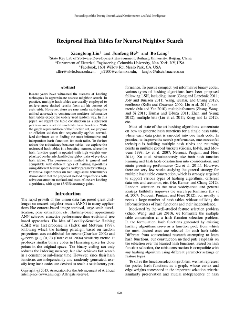
Figure 1 demonstrates the proposed table construction
method that reciprocally selects dominant hashing functions
in a boosting manner. Our empirical study on several largescale benchmarks highlights the benefits of our method,
with significant performance gains over the popular random
selection and several state-of-the-art hashing algorithms.
Graph Representation
Motivated by recent research on modelling correlations
based on graph (Pavan and Pelillo 2007; Liu and Yan 2010),
we first represent the pooled hash functions H as a vertexweighted and undirected edge-weighted graph:
G = (V, E, A, π).
(1)
Problem Definition
V = {1, . . . , B} is the vertex set corresponding to the
B hash functions in H with weights π = [π1 , . . . , πB ]T .
E ⊆ V × V is the edge set with weights A = (aij ), whose
entry aij : (i, j) ∈ E → R∗ is a non-negative weight
corresponding to the edge between vertex i and j.
The vertex weights characterize the quality of each hash
function, while the edge weights describe the pairwise relationships between hash functions (in practice it is difficult
to compute higher-order correlations among more than two
hash functions). Prior hashing research has proved that
similarity preservation of each hash function and independence among them are two satisfying, yet non-redundant
criteria for compact hash code generation in a single hash
table (Weiss, Torralba, and Fergus 2008; Wang, Kumar, and
Chang 2012). Therefore, we respectively adopt them as the
vertex and edge weights in graph G.
Suppose we have a pool of B hash functions
H = {h1 (·), . . . , hB (·)} with the index set V = {1, . . . , B},
each of which is a binary mapping hi (·) : Rd → {−1, 1}.
These hash functions can be generated by different types
of hashing algorithms (linear/nonlinear, random/optimized,
etc.) with different features, parameter settings, etc.
Vertex Weights To obtain good hash codes guaranteeing
search accuracy, hash functions should preserve similarities
between data points, namely, neighbor points are supposed
to have similar hash codes (Weiss, Torralba, and Fergus
2008), and non-neighbor pairs should be separated with a
large margin (Wang, Kumar, and Chang 2012). To assess
such capability of each hash function, a reasonable criteria
Notations
627
Algorithm 1 Hash Table Construction using Dominant
Hash Functions (DHF).
1: Input: data X, hash function set H, similarity S;
2: Initialize: Yi ← hi (X), i = 1, . . . , B;
3: Compute weights π and A by Eq. (3) and Eq. (4);
4: for l = 1 to L do
5:
Optimize z∗ of problem (5) with respect to H;
6:
Set σ ← topK(z∗ ) and V ← {1, . . . , |H|} \ σ;
7:
Set Tl ← {hi : hi∈σ ∈ H};
8:
Update H ← H \ Tl and A ← AV ;
9: end for
10: Output: hash tables Tl , l = 1, . . . , L.
is the empirical accuracy (Wang, Kumar, and Chang 2012),
the difference between the numbers of correctly and wrongly
classified neighbors by each hash function. It relies on
two types of neighbor sets: homogenous neighbors M and
heterogeneous neighbors C (Yan et al. 2007). If i-th and jth samples are either nearest neighbors in a metric space or
share common labels, then (i, j) ∈ M. Similarly, if they
are far away or have different labels, then (i, j) ∈ C. The
similarity matrix S will be
1, if (i, j) ∈ M
−1, if (i, j) ∈ C
Sij =
(2)
0, otherwise
Based on the predefined similarity matrix S, we define
the vertex weight of the i-th hash function in terms of the
similarity preservation, with a γ > 0:
(3)
πi = exp γYi SYiT .
Theorem 1 If z∗ is a strict local solution of the program
max
s.t.
z ≥ 0, 1 z = 1
(5)
where  = ΠAΠ, and Π = diag(π), then its support
σ(z∗ ) = {i ∈ V : zi∗ = 0} is the normalized dominant
set of graph G = (V, E, A, π).
Edge Weights Previous research shows that the independent hash functions are desired to generate compact binary
codes (Weiss, Torralba, and Fergus 2008). Mutual information among their bit variables serves as a good independence
criterion (He et al. 2011). Following (Heo et al. 2012), we
approximate it by considering the pairwise case .
Given the bit distribution for i-th hash function p(yi ), yi ∈
{−1, 1}, and the joint bit distribution for i-th and j-th
functions p(yi , yj ), the independence aij between any i-th
and j-th bits based on their mutual information forms the
edge weights A = (aij ), and each aij is defined with a
λ > 0:
⎤
⎡
,
y
)
p(y
i j ⎦
. (4)
p(yi , yj ) log
aij = exp ⎣−λ
p(y
)p(y
i
j)
y ,y
i
1 T
2 z Âz
T
Theorem 1 indicates that the dominant set can be found
efficiently by solving the quadratic programming problem
in (5), whose strict and stable solution with respect to the
nonnegative and symmetric  can be optimized using the
replicator dynamics (Pavan and Pelillo 2007; Liu and Yan
2010) with the following iterations:
zi (t + 1) = zi (t)
(Âz(t))i
z(t)T Âz(t)
, i = 1, . . . , L.
(6)
The objective function 12 zT Âz of program (5) reflects
the cohesiveness among functions, incorporating both proposed selection criteria. The solution z∗ naturally scores
each function, and its nonzero elements correspond to the
dominant set in G. Then, our dominant hash functions are
the K functions indexed by topK(z∗ ) with highest scores in
H, which directly constitutes an informative hash table.
Based on the idea of dominant hash functions, our
straightforward strategy for hash table construction is to
iteratively solve similar problems in (5), with respect to
the remaining unselected hash functions (those already
selected in previous tables are removed from H). Algorithm
1 (named DHF for short) outlines the detailed table
construction procedure using dominant hash functions,
where AV denotes the submatrix of A with the rows and
the columns indexed by the elements of V. The algorithm
is feasible for large-scale problems, since A can be sparse,
and efficient optimization methods like graph shift (Liu and
Yan 2010) can be adopted for fast computation.
j
Here aii = 0, because each function is self-dependent.
Informative Hash Table
Similarity preservation measures each hash function’s capability of retaining neighbor relationships, while their independence results in short, yet discriminative hash codes
by reducing the redundancy among them. To achieve high
performance, the hash functions that are not only capable of preserving neighbor relationships but also mutually
independent should be selected for an informative hash
table. This intuition indicates that the most desired subset of
hash functions should possess high vertex and edge weights
inside, and thus can be regarded as the dominant set on the
graph G (Pavan and Pelillo 2007; Liu and Yan 2010).
In the dominant set, each element is associated with a
discriminative score induced from both vertex and edge
weights. Therefore, the most desired K hash functions
(named dominant hash functions) from the candidate set
H are equivalent to the elements with largest scores in the
dominant set of graph G. We establish the following theorem
that explores the efficient solution to the dominant set (Liu
et al. 2013):
Reciprocal Hash Tables
Although Algorithm 1 selects the most independent and
informative functions for each hash table, it still ignores the
redundancy among tables. In practice, it is critical that the
multiple tables can be complementary to each other (Xu et
al. 2011; He et al. 2011), so that the nearest neighbors can be
628
Algorithm 2 Reciprocal Hash Table Construction using
Dominant Hash Functions (RDHF).
1: Input: data X, hash function set H, similarity S;
2: Initialize: Yi ← hi (X), i = 1, . . . , B;
3: Compute edge weights A by Eq. (4);
4: for l = 1 to L do
5:
Update ωij and Sij by Eq. (9) and Eq. (10);
6:
Compute vertex weights π by Eq. (3);
7:
Optimize z∗ of problem (5) with respect to H;
8:
Set σ ← topK(z∗ ) and V ← {1, . . . , |H|} \ σ;
9:
Set Tl ← {hi : hi∈σ ∈ H};
10:
Update H ← H \ Tl and A ← AV ;
11: end for
12: Output: hash tables Tl , l = 1, . . . , L.
found in at least one of them. To take the factor into account,
we construct reciprocal hash tables in a boosting manner,
which sequentially selects the dominant hash functions that
well separate the previous misclassified neighbor pairs.
In the boosting framework, we consider the neighbor
prediction of multiple hash tables with respect to the two
types of neighbors. Let’s define the prediction of the current
l hash tables on the neighbor pair xi and xj as
pij = dlij − μ,
(7)
dlij
where
is the hamming distance contributed from l hash
tables (let d0ij = 0):
dlij = min
h(xi ) − h(xj )2 ,
(8)
i=1,...,l
h∈Ti
and μ is the average hamming distance of all neighbors.
In each round, a new hash table is constructed by selecting
the hash functions that can correct the prediction errors of
previous tables. Therefore, the weights on the misclassified
neighbor pairs will be amplified to incur greater penalty,
while those on the correctly classified ones will be shrunk.
Specifically, in the l-th round the weights ω are updated
based on the prediction p of previous (l − 1) tables:
exp(−αpij ), if (i, j) ∈ M
exp(αpij ), if (i, j) ∈ C
ωij =
(9)
0,
otherwise
Data Sets and Protocols
We conduct experiments on two widely-used large data sets
in hashing research: SIFT-1M and GIST-1M, consisting of
one million 128-D SIFT and 960-D GIST features respectively (Jegou, Douze, and Schmid 2011). For each data set,
we construct a training set of 10,000 random samples and a
test query set of 1,000 ones. We consider metric neighbors in
the similarity matrix, where 100 homogenous neighbors and
200 heterogenous neighbors are calculated for each training
sample (Yan et al. 2007). The groundtruth for each query is
defined as the top 5 nearest neighbors computed by the
exhaustive linear scan based on Euclidean distances.
Two common search methods are adopted in the evaluation, including Hamming ranking and hash lookup. The
former ranks all points in the database according to their
Hamming distances (Equation 8) from the query, while the
later retrieves all points falling in the buckets of all tables
within certain Hamming radius (usually 2) from the query
codes.
All experiments are conducted on a workstation with Intel
Xeon CPU E5645@2.40GHz and 24GB memory, and the
results reported in this paper are averaged over 10 runs. For
parameter (γ and λ) sensitivity, we observe that the proposed
method is relatively robust to them. Thus, we roughly fix
γ = 0.2 and λ = 4 in all experiments.
I(pij Sij <0)
where α = ln ij I(pij Sij ≥0) , measuring the total error rate
ij
of all (l − 1) hash tables, and I(·) is the indicator function.
The weight updating takes account of both the neighbor
prediction on each pair and the overall prediction error of
previous tables. Then, a typical way to update the similarity
matrix S will be
Sij = Sij ωij .
(10)
The updating scheme enlarges the similarity magnitudes
of incorrectly predicted neighbor pairs compared to others.
Based on S, the hash functions that well preserve the misclassified neighbors will gain large vertex weights updated
using (3). Therefore, they possess high priority to be selected
as the dominant hash function for the new hash table.
In Algorithm 2 (RDHF) we give our construction approach to reciprocal hash tables using dominant hash functions (See the illustration of the constructing procedure in
Figure 1). Compared with DHF, RDHF requires to update
the similarity matrix in each round, however, the extra
computation is actually very small because of its sparsity.
Over Basic Hashing Algorithms
The proposed table construction methods as well as the random way can support any types of hashing algorithms (e.g.,
linear/nonlinear, random/optimized). Next, we comprehensively evaluate them over several basic hashing algorithms
in terms of both hash lookup and Hamming ranking.
Experiments
In this section we will evaluate multiple table construction
methods for two useful scenarios, that the hash functions
are generated using basic hashing algorithms and multiple
multi-bit hashing algorithms respectively. The proposed
method based on dominant hash functions (DHF) and its reciprocal version (RDHF) will be compared with the random
selection (RAND, the only general construction method in
the literature) on several datasets. It should be noted that
the performance of all these methods relies on the source
hashing algorithms that generate the pooled hash functions.
Hash Lookup Evaluation Hash For fast computation,
state-of-the-art hashing algorithms usually build several
hash tables and lookup multiple buckets (Lv et al. 2007;
Norouzi, Punjani, and Fleet 2012) to retrieve more desired
points, which however sharply reduces the search accuracy
due to a large portion of irrelevant points contained in
them (see an example in Table 1, where using 1 table
and 8 tables the recall performance increases from 7.03%
to 31.94%, but the precision decreases from 21.91% to
629
Table 1: PH2 (%) of multiple LSH hash tables on SIFT-1M.
# TABLES→
RAND
DHF
RDHF
1
21.91
26.29
26.29
4
18.29
28.87
29.25
8
16.20
26.88
27.60
12
14.42
23.24
23.80
Table 3: Performance (%) of hash lookup within Hamming
radius 2 using multiple hashing tables on GIST-1M.
16
13.15
16.22
16.44
8
8.42
8.93
9.34
7.36
11.32
PCAR DB
ITQ DB
RAND
DHF
RDHF
16.20%). By contrast, our method relieves the degeneration
by complementarily constructing multiple hash tables using
the most informative and independent hash functions. On
the one hand, each hash table is discriminative enough to
find parts of the true neighbors; on the other hand, reciprocal
hash tables together are able to widely cover all parts of
neighbors.
Table 1 lists the hash lookup results (precision within
hamming radius less than 2 (PH2)) comparing our methods
(DHF and RDHF) with conventional random way (RAND).
We build a function pool containing 500 Locality Sensitive
Hashing (LSH) (Datar et al. 2004) functions on SIFT-1M.
Using each construction method, we respectively construct
a different number of hash tables, each of which consists
of 24 (close to the optimal value log2 n for n = 106
points) hash functions (Norouzi, Punjani, and Fleet 2012;
Slaney, Lifshits, and He 2012). It is obvious that the precision of RAND deceases dramatically with more hash tables,
while (R)DHF increase their performance first and attain
significant performance gains over RAND in all cases.
In addition to LSH (linear, random), we also investigate
the performance using other basic hashing algorithms including Kernelized LSH (KLSH) (Kulis and Grauman 2009)
(non-linear,random) and Random Maximum Margin Hashing (RMMH) (Joly and Buisson 2011) (linear, optimized).
Table 2 shows their PH2 performance using 8, 12, and 16
hash tables on SIFT-1M and GIST-1M. From the table,
we first observe that DHF consistently outperforms RAND
using different hashing algorithms, with large performance
margins (e.g., 65.93%, 56.10%, and 22.48% using 8 LSH,
KLSH, and RMMH hash tables respectively on SIFT-1M).
Moreover, owing to the complementary relationships among
the hash tables, RDHF is slightly better than DHF in most
cases, especially using more hash tables. It should be noted
that PH2 performance of both DHF and RDHF drops faster
than RAND when using more hash tables. This is because
that DHF and RDHF construct hash tables by sequentially
selecting the most informative functions, and thus the quality of their tables will decrease slightly. Even so, in all
cases both methods faithfully improve the performance over
RAND in terms of hash lookup.
P RECISION
12
8.41
8.72
9.26
7.13
10.82
16
8.31
8.60
9.10
6.98
10.44
8
4.90
5.24
5.82
1.11
6.89
R ECALL
12
5.79
6.50
7.01
2.12
9.40
16
6.74
7.57
8.19
3.37
10.88
0.14
precision@1000
0.12
0.1
0.08
0.06
PCARDB
ITQDB
RAND
DHF
RDHF
0.04
0.02
0
8 tables
12 tables
16 tables
Figure 3: Hamming ranking precisions using multiple double bit hashing algorithms on GIST-1M.
independence of hash functions, consistently achieve the
best performance over LSH, KLSH and RMMH in most
cases (e.g., on SIFT-1M, DFH using 12 tables gets 18.73%,
11.86%, and 7.58% precision@1,000 gains over RAND),
and RDHF gains significant performance improvements
over DHF by exploiting the mutual benefits between tables.
Moreover, we can conclude that both methods can increase
their performance using more hash tables (e.g., for RDHF on
GIST-1M, the precision@1,000 gain is up to 9.00%), while
RAND improves very little, due to its aimless selection.
Over Multiple Hashing Algorithms
As mentioned earlier, there exist various situations that we
need build multiple hash tables using different hashing algorithms with different settings. Besides the simple scenario in
the last section, here we verify that our construction method
can also work well with more complex scenarios, e.g.,
construction using multiple double-bit hashing algorithms.
In practice, many hashing algorithms are prevented from
being directly used to construct multiple tables, due to the
upper limit of the hash function number, stemming from
the dimension of data representation (e.g., Iterative Quantization (Gong and Lazebnik 2011) can generate no more
than 128 functions using SIFT feature). Table construction
using multiple double-bit hashing algorithms can tackle this
problem using double bit hashing algorithms like (Liu et al.
2011) and (Kong and Li 2012), which generate multiple hash
functions along a single projection. However, the quality
of these functions varies in a wide range, especially using
hierarchical quantization (Liu et al. 2011).
We evaluate our method in this scenario to demonstrate
that how it efficiently picks the high quality hash functions
for table construction. In this experiment, a 1,000 hash func-
Hamming Ranking Evaluation Hamming ranking usually achieves efficient implementation using the fast binary
operations, and thus has been widely employed in hashing
based ANN search (Liu et al. 2011; Xu et al. 2011; Wang,
Kumar, and Chang 2012). We study the Hamming ranking
performance of all three construction methods, and plot the
precision curves in Figure 2. Here RAND is actually equivalent to multi-index hashing (MIH) (Norouzi, Punjani, and
Fleet 2012), since these basic hashing algorithms generate
their hashing functions disorderly and independently.
From Figure 2, it can be easily observed that DHF
and RDHF, considering similarity preservation and mutual
630
Table 2: PH2 (%) of multiple hashing tables over LSH, KLSH, and RMMH on GIST-1M and SIFT-1M.
A LGORITHMS →
# TABLES →
RAND
DFH
RDFH
RAND
DFH
RDFH
SIFT-1M
GIST-1M
KLSH
12
17.46
25.34
26.00
11.20
13.63
14.00
16
16.09
18.86
19.45
10.73
11.88
12.31
0.35
0.3
0.25
0.4
0.3
200
400
600
800
0.25
0
1000
200
400
600
800
0
0.12
0.11
0.1
400
600
800
1000
(c) Precision of RMMH on SIFT-1M
0.24
0.2
0.18
0.16
RAND 8 tables
RAND 12 tables
DHF 8 tables
DHF 12 tables
RDHF 8 tables
RDHF 12 tables
0.22
precision
0.13
200
number of top retrieved samples
RAND 8 tables
RAND 12 tables
DHF 8 tables
DHF 12 tables
RDHF 8 tables
RDHF 12 tables
0.22
precision
0.14
0.4
1000
0.24
RAND 8 tables
RAND 12 tables
DHF 8 tables
DHF 12 tables
RDHF 8 tables
RDHF 12 tables
0.15
RAND 8 tables
RAND 12 tables
DHF 8 tables
DHF 12 tables
RDHF 8 tables
RDHF 12 tables
0.35
(b) Precision of KLSH on SIFT-1M
0.16
16
23.73
28.63
29.16
10.58
11.59
12.04
0.45
number of top retrieved samples
(a) Precision of LSH on SIFT-1M
RMMH
12
24.87
30.62
30.95
10.96
12.68
13.03
0.5
0.35
number of top retrieved samples
8
26.02
31.87
31.23
11.58
13.28
13.45
0.55
RAND 8 tables
RAND 12 tables
DHF 8 tables
DHF 12 tables
RDHF 8 tables
RDHF 12 tables
0.45
precision
precision
8
19.20
29.97
29.40
11.83
14.37
14.27
0.5
RAND 8 tables
RAND 12 tables
DHF 8 tables
DHF 12 tables
RDHF 8 tables
RDHF 12 tables
0.4
precision
16
13.15
16.22
16.44
8.24
8.72
8.99
precision
0.45
0.2
0
LSH
12
14.42
23.24
23.80
8.51
9.30
9.67
8
16.20
26.88
27.60
8.80
9.21
9.68
0.2
0.18
0.16
0.09
0.08
0
200
400
600
800
1000
number of top retrieved samples
(d) Precision of LSH on GIST-1M
0
200
400
600
800
1000
number of top retrieved samples
(e) Precision of KLSH on GIST-1M
0
200
400
600
800
1000
number of top retrieved samples
(f) Precision of RMMH on GIST-1M
Figure 2: Hamming ranking performance of multiple table methods over basic hashing algorithms on SIFT-1M and GIST-1M.
tion pool is equally generated on GIST-1M by double bit
(DB) quantization (Liu et al. 2011) on PCA-based Random
Rotation Hashing (PCARDB) and Iterative Quantization
(ITQDB) (Gong and Lazebnik 2011). Table 3 reports both
precision and recall performance of all construction methods
using hash lookup. Compared with the basic DB methods,
RAND gives a balanced performance between them. But
our RDFH, filtering poor quality functions out, significantly
boosts the performance over these baselines with more than
14.73% precision and 18.38% recall gains. We also show
their Hamming ranking performance in Figure 3, where
we obtain the same conclusion that RDFH significantly
outperforms others using a varying number of hash tables.
well on the misclassified neighbors, and thus achieves the
best performance.
Conclusion
We proposed a unified strategy for hash table construction supporting different hashing algorithms and various
scenarios. For each table, its hash functions correspond
to the dominant set in a vertex- and edge-weighted graph
representing all pooled hash functions. These dominant
hash functions are mutually uncorrelated, and preserve data
similarities well. To reduce the redundancy between hash
tables, we presented a reciprocal strategy based on dominant
hash functions. It sequentially explores a new hash table to
compensate the mistakes of pervious tables in a boosting
manner. Comprehensive evaluation on large-scale benchmarks shows the strong practicability and the encouraging
performances.
Note that DHF fails to compete with the baselines. According to our observations, this is because the hashing
functions of DFH mostly come from the second functions of
each projection, which individually lower the quantization
loss (Kong and Li 2012), but break the neighbor relationships as a table. On the contrary, for each table RDHF
adaptively prefers the high-quality hash functions that work
631
Acknowledgments
hashing. In IEEE International Conference on Computer
Vision and Pattern Recognition.
Lv, Q.; Josephson, W.; Wang, Z.; Charikar, M.; and Li,
K. 2007. Multi-probe lsh: efficient indexing for highdimensional similarity search. In Proceedings of the 33rd
international conference on Very large data bases, 950–961.
Mu, Y., and Yan, S. 2010. Non-metric locality-sensitive
hashing. In Fox, M., and Poole, D., eds., AAAI Conference
on Artificial Intelligence. AAAI Press.
Norouzi, M.; Punjani, A.; and Fleet, D. J. 2012. Fast
search in hamming space with multi-index hashing. In IEEE
Conference on Computer Vision and Pattern Recognition,
3108–3115.
Pavan, M., and Pelillo, M. 2007. Dominant sets and pairwise
clustering. IEEE Trans. Pattern Anal. Mach. Intell. 167–172.
Slaney, M.; Lifshits, Y.; and He, J. 2012. Optimal
parameters for locality-sensitive hashing. Proceedings of the
IEEE 100(9):2604–2623.
Wang, J.; Kumar, S.; and Chang, S.-F. 2012. Semisupervised hashing for large scale search. Pattern Analysis
and Machine Intelligence, IEEE Transactions on.
Weiss, Y.; Torralba, A.; and Fergus, R. 2008. Spectral
hashing. In Advances in Neural Information Processing
Systems.
Xu, H.; Wang, J.; Li, Z.; Zeng, G.; Li, S.; and Yu, N. 2011.
Complementary hashing for approximate nearest neighbor
search. In IEEE International Conference on Computer
Vision.
Yan, S.; Xu, D.; Zhang, B.; Zhang, H.; Yang, Q.; and Lin, S.
2007. Graph embedding and extensions: A general framework for dimensionality reduction. IEEE Trans. Pattern
Anal. Mach. Intell. 29(1):40–51.
Zhang, D.; Wang, F.; and Si, L. 2011. Composite hashing with multiple information sources. In ACM SIGIR
Conference on Research and Development in Information
Retrieval.
Zhao, Z.; Wang, L.; and Liu, H. 2010. Efficient spectral
feature selection with minimum redundancy. In AAAI
Conference on Artificial Intelligence.
Zhen, Y., and Yeung, D.-Y. 2012. Co-regularized hashing
for multimodal data. In Advances in Neural Information
Processing Systems.
. This work is supported by National Major Project of China
(2010ZX01042-002-001-00) and the SKLSDE Foundation
(SKLSDE-2011ZX-01).
References
Charikar, M. S. 2002. Similarity estimation techniques
from rounding algorithms. ACM Symposium on Theory of
Computing, 380–388. New York, NY, USA: ACM.
Datar, M.; Immorlica, N.; Indyk, P.; and Mirrokni, V. S.
2004. Locality-sensitive hashing scheme based on p-stable
distributions. In Symposium on Computational Geometry.
Gionis, A.; Indyk, P.; and Motwani, R. 1999. Similarity
search in high dimensions via hashing. In Very Large Data
Bases.
Gong, Y., and Lazebnik, S. 2011. Iterative quantization:
A procrustean approach to learning binary codes. In IEEE
International Conference on Computer Vision and Pattern
Recognition, 817 –824.
He, J.; Chang, S.-F.; Radhakrishnan, R.; and Bauer, C. 2011.
Compact hashing with joint optimization of search accuracy
and time. In IEEE International Conference on Computer
Vision and Pattern Recognition, 753–760.
He, J.; Kumar, S.; and Chang, S.-F. 2012. On the difficulty
of nearest neighbor search. In International Conference on
Machine Learning.
Heo, J.-P.; Lee, Y.; He, J.; Chang, S.-F.; and Yoon, S.-E.
2012. Spherical hashing. In IEEE International Conference
on Computer Vision and Pattern Recognition, 2957–2964.
Indyk, P., and Motwani, R. 1998. Approximate nearest
neighbors: towards removing the curse of dimensionality. In
ACM Symposium on Theory of Computing.
Jegou, H.; Douze, M.; and Schmid, C. 2011. Product
quantization for nearest neighbor search. IEEE Trans.
Pattern Anal. Mach. Intell. 33(1):117–128.
Joly, A., and Buisson, O. 2011. Random maximum margin
hashing. In IEEE International Conference on Computer
Vision and Pattern Recognition, 873–880.
Kong, W., and Li, W.-J. 2012. Double-bit quantization for
hashing. In AAAI Conference on Artificial Intelligence.
Kulis, B., and Grauman, K. 2009. Kernelized localitysensitive hashing for scalable image search. In IEEE
International Conference on Computer Vision.
Kumar, S., and Udupa, R. 2011. Learning hash functions
for cross-view similarity search. In Proceedings of the
Twenty-Second international joint conference on Artificial
Intelligence, 1360–1365. AAAI Press.
Liu, H., and Yan, S. 2010. Robust graph mode seeking
by graph shift. In International Conference on Machine
Learning, 671–678.
Liu, W.; Wang, J.; Kumar, S.; and Chang, S.-F. 2011. Hashing with graphs. In International Conference on Machine
Learning.
Liu, X.; He, J.; Lang, B.; and Chang, S.-F. 2013. Hash
bit selection: a unified solution for selection problems in
632