Proceedings of the Twenty-Ninth AAAI Conference on Artificial Intelligence
How Many Diagnoses Do We Need?
Roni Stern and Meir Kalech and Shelly Rogov
Alexander Feldman
Ben Gurion University of the Negev
Be’er Sheva, Israel
Palo Alto Research Center
Palo Alto, CA, USA
Abstract
C1
A known limitation of many diagnosis algorithms is that
the number of diagnoses they return can be very large.
This raises the question of how to use such a large set
of diagnoses. For example, presenting hundreds of diagnoses to a human operator (charged with repairing the
system) is meaningless. In various settings, including
decision support for a human operator and automated
troubleshooting processes, it is sufficient to be able to
answer a basic diagnostic question: is a given component faulty? We propose a way to aggregate an arbitrarily large set of diagnoses to return an estimate of the
likelihood of a given component to be faulty. The resulting mapping of components to their likelihood of
being faulty is called the system’s health state. We propose two metrics for evaluating the accuracy of a health
state and show that an accurate health state can be found
without finding all diagnoses. An empirical study explores the question of how many diagnoses are needed
to obtain an accurate enough health state, and a simple
online stopping criterion is proposed.
C2
In
p({C1,C2})=0.2
Out
C3
C4
p({C3,C4})=0.16
C5
p({C3,C5})=0.16
C6
p({C3,C6})=0.16
C7
p({C3,C7})=0.16
C8
p({C3,C8})=0.16
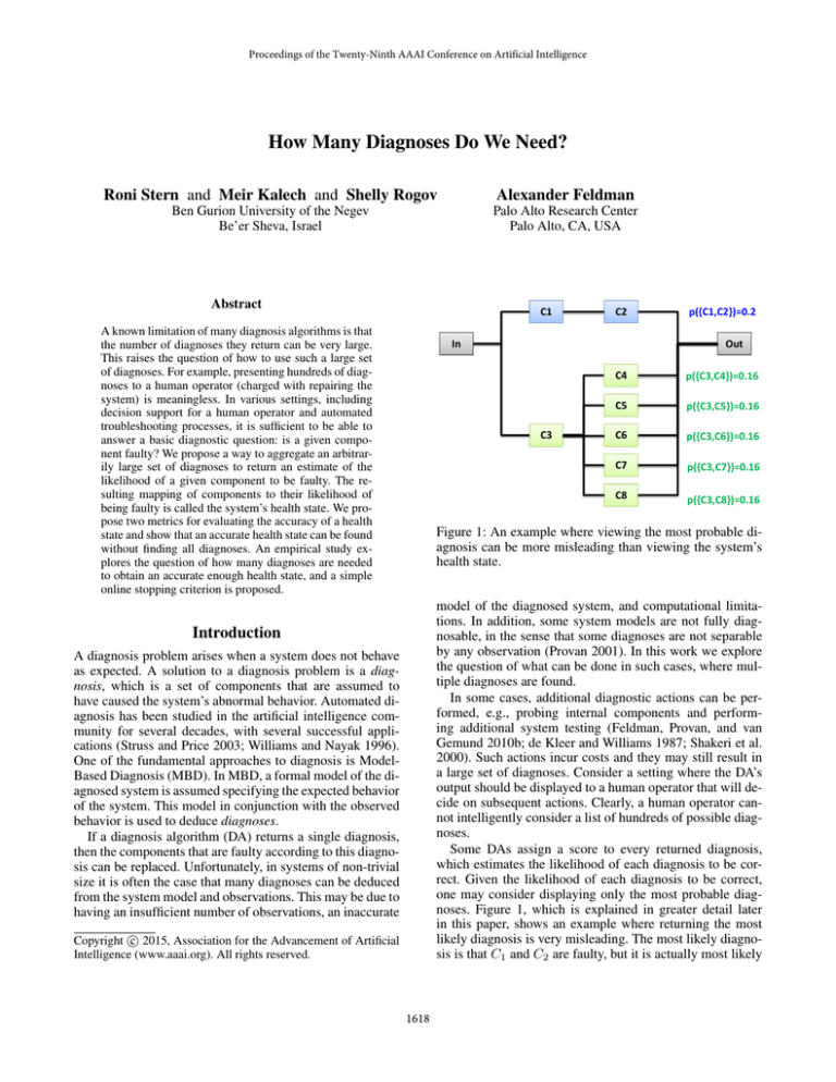
Figure 1: An example where viewing the most probable diagnosis can be more misleading than viewing the system’s
health state.
model of the diagnosed system, and computational limitations. In addition, some system models are not fully diagnosable, in the sense that some diagnoses are not separable
by any observation (Provan 2001). In this work we explore
the question of what can be done in such cases, where multiple diagnoses are found.
In some cases, additional diagnostic actions can be performed, e.g., probing internal components and performing additional system testing (Feldman, Provan, and van
Gemund 2010b; de Kleer and Williams 1987; Shakeri et al.
2000). Such actions incur costs and they may still result in
a large set of diagnoses. Consider a setting where the DA’s
output should be displayed to a human operator that will decide on subsequent actions. Clearly, a human operator cannot intelligently consider a list of hundreds of possible diagnoses.
Some DAs assign a score to every returned diagnosis,
which estimates the likelihood of each diagnosis to be correct. Given the likelihood of each diagnosis to be correct,
one may consider displaying only the most probable diagnoses. Figure 1, which is explained in greater detail later
in this paper, shows an example where returning the most
likely diagnosis is very misleading. The most likely diagnosis is that C1 and C2 are faulty, but it is actually most likely
Introduction
A diagnosis problem arises when a system does not behave
as expected. A solution to a diagnosis problem is a diagnosis, which is a set of components that are assumed to
have caused the system’s abnormal behavior. Automated diagnosis has been studied in the artificial intelligence community for several decades, with several successful applications (Struss and Price 2003; Williams and Nayak 1996).
One of the fundamental approaches to diagnosis is ModelBased Diagnosis (MBD). In MBD, a formal model of the diagnosed system is assumed specifying the expected behavior
of the system. This model in conjunction with the observed
behavior is used to deduce diagnoses.
If a diagnosis algorithm (DA) returns a single diagnosis,
then the components that are faulty according to this diagnosis can be replaced. Unfortunately, in systems of non-trivial
size it is often the case that many diagnoses can be deduced
from the system model and observations. This may be due to
having an insufficient number of observations, an inaccurate
Copyright c 2015, Association for the Advancement of Artificial
Intelligence (www.aaai.org). All rights reserved.
1618
that C3 and one of the components after it is faulty. Thus,
while showing a long list of diagnoses to a human operator is not helpful, focusing on a single diagnosis may miss
important diagnostic information.
Our first contribution is in proposing to aggregate the set
of diagnoses into a single vector containing for every component the likelihood that it is faulty. We call this vector
the system’s health state. To a human operator a system’s
health state provides a manageable view of which components are likely to be faulty. A notion similar to health states
has been used for automated troubleshooting (Zamir, Stern,
and Kalech 2014).
A health state can be derived from an arbitrarily large
set of diagnoses and their likelihoods. In this work we investigate experimentally the relation between the accuracy
of a health state and the number and type of diagnoses
used to generate it. The second contribution of this work
is in proposing two metrics for measuring the quality of
a health state. The first metric is based on Euclidean distance from the optimal health state (where the true faults are
known). The second metric views a health state as a classifier’s model, and measures its quality according to the area
under the curve (AUC) of a receiver operating characteristic (ROC) curve. Under both quality metrics, we observed
empirically that the quality of a health state converges to a
stable value without finding all diagnoses. This stable value
is shown to be close to the best quality achievable, and that
in most cases such a value can be obtained by considering
only minimal cardinality diagnoses (diagnoses with a minimal number of faulty components). This supports the common diagnosis approach of focusing first on diagnoses with
lower cardinality.
The empirical evaluation also shows that in most cases
only a fraction of the set of minimal cardinality diagnoses is
needed in order to reach a health state with a stable value.
This result opens a great opportunity to develop DAs that
determine online when to stop searching for more diagnoses (Feldman, Janssen, and van Gemund 2011). An online
stopping condition for such an algorithm is proposed with
promising preliminary results, suggesting future research.
fault models (WFMs) and strong fault models (SFMs),
where in WFMs only the nominal behavior a component
is specified and in SFMs additional information is available
about how faulty components behave. For ease of presentation, we assume in this paper a WFM, but all the theoretical
results can be generalized to a SFM.
Figure 2 shows an example of an MBD problem, where
the normal behavior would give output E = 1 but the observation had E = 0. DAs try to find diagnoses, which are
subsets of COMPS that explain the observation if assumed
faulty.
Definition 1 (Diagnosis). A set of components ! ✓
is a diagnosis if the following term is consistent
^
^
SD ^
¬h(c) ^
h(c) ^ OBS
c2!
COMPS
c2!
/
We say that ! is a minimal diagnosis if no proper subset ! 0 ⇢
! is a diagnosis, and that ! is a minimal cardinality diagnosis if
no other diagnosis ! 0 ✓ COMPS exists such that |! 0 | < |!|.
= {X1 , X2 , A1 , A2 , O1 }
= {A, ¬B, C, ¬D, ¬E}
COMPS
OBS
Figure 2: MBD: A full adder.
For the MBD problem in Figure 2, !1 ={X1 , X2 },
!2 ={O1 }, !3 ={A2 } are all the minimal diagnoses, and
!2 , !3 are all the minimal cardinality diagnoses. Some
DAs search for subset-minimal diagnoses (Stern et al. 2012;
de Kleer and Williams 1987; Williams and Ragno 2007)
and other DAs search only for minimal cardinality diagnoses (Metodi et al. 2012; de Kleer 2009). Finding a single
minimal cardinality diagnosis is an NP-hard problem (Selman and Levesque 1990) and finding more than one subsetminimal diagnosis is also NP-hard (Bylander et al. 1991).
Even if limiting the output of a DA to only return minimal
cardinality diagnoses, the number of returned diagnoses can
still be exponential in the size of the diagnosis cardinality
(the number of components assumed to be faulty). This occurs in practice in standard MBD benchmarks (Siddiqi 2011;
Metodi et al. 2012). The question of how to manage such a
large set of output diagnoses still holds, even if limiting the
set of diagnoses to only include minimal cardinality diagnoses.
Model Based Diagnosis
An MBD problem is specified as a triplet hSD, COMPS , OBS i
where: SD is a model of the diagnosed system, COMPS is a
set of components, and OBS is an observation.
SD takes into account that some components might be abnormal (faulty). This is specified by an unary predicate h(·),
such that h(c) and ¬h(c) denote that component c is healthy
or faulty, respectively. Denoting the correct behavior of component c as a propositional formula, 'c , SD is given formally
as
^
SD =
(h(c) ! 'c )
Health States
Given a large set of diagnoses, a reasonable question that
a human operator might ask is “what is the likelihood that
a component C is faulty?” This is helpful, for example, to
decide which component to replace first. In addition, being able to estimate the likelihood of each component being faulty is helpful in troubleshooting algorithms (Zamir,
c2COMPS
Namely, a healthy component follows its correct behavior.
A diagnosis problem (DP) arises when the assumption that
all components are healthy is inconsistent with the system
description and observation (de Kleer and Williams 1987;
Reiter 1987). System models can be classified into weak
1619
Stern, and Kalech 2014; Heckerman, Breese, and Rommelse
1995).
Definition 2 (Health State). A health state is a vector H 2
[0, 1]|COMPS| where the ith element of H, denoted H[i], is
an estimate of the likelihood that component Ci 2 COMPS is
faulty.
Next, we show how a health state can be generated from
a set of diagnoses (found by a DA).
Let ⌦ be a set of diagnoses found by a DA, and let
p : ⌦ ! [0, 1] be a probability distribution over the diagnoses in ⌦, such that p(!) corresponds to the probability
! 2 ⌦ is correct. Many DAs prioritize the diagnoses in ⌦,
and some return a score for each diagnosis to denote how
likely it is to be correct (Abreu et al. 2009). A common
method to generate such a score is by considering a prior
probability on the fault of each component (without considering the observations), and assuming that components fail
independently. This is a common assumption in MBD (de
Kleer and Williams 1987; Williams and
Q Ragno 2007). Thus,
a score of a diagnosis ! would be Ci 2! pr(Ci ), where
pr(Ci ) is the prior probability that Ci is faulty. Converting
diagnoses scores to a valid probability distribution simply
requires normalizing their sum to one:
Q
Ci 2! pr(Ci )
Q
p(!) = P
! 0 2⌦
Ci 2! 0 pr(Ci )
C1
C2
C3
C4
C5
C6
C7
C8
p
!3
0
0
1
0
1
0
0
0
0.16
!4
0
0
1
0
0
1
0
0
0.16
!5
0
0
1
0
0
0
1
0
0.16
!6
0
0
1
0
0
0
0
1
0.16
H[i]
0.2
0.2
0.8
0.16
0.16
0.16
0.16
0.16
{C1 , C2 }, having a probability of 0.2. The health state, however, point at C3 as the component that is most likely to be
faulty, having H[3] = 0.8.
While a health state is an informative aggregation of a
given set of diagnoses, some information contained in the
set of diagnoses it was generated from, is lost. This lost information is the dependencies between the different components. For example, consider again the diagnoses in Figure 1.
The component C1 is only a member of a single diagnosis
{C1 , C2 }. Thus, repairing only C1 without repairing C2 is
not likely to fix the system. This relation between C1 and
C2 is lost in the aggregated perspective of a health state.
Automated troubleshooting algorithms (Feldman, Provan,
and van Gemund 2010b; de Kleer and Williams 1987;
Shakeri et al. 2000) might make use of such additional relation information and might thus prefer as input a list of
diagnoses over a health state.
Evaluating a Health State
!2⌦
Ci 2!
!2
0
0
1
1
0
0
0
0
0.16
Table 1: Diagnoses and health state for Figure 1
Other methods to generate a probability distribution p over
⌦ may also exist.
Given ⌦ and p, we can derive a health state as follows:
X
H[i] =
p(!) · Ci 2!
(1)
where
!1
1
1
0
0
0
0
0
0
0.2
is the indicator function defined as:
⇢
1
Ci 2 !
Ci 2! =
0 otherwise
Due to computational limitations, DAs often cannot return
all the diagnoses for a given diagnosis problem. In addition,
the diagnosis likelihood function p is often a (usually rough)
approximation. This raises the question of how accurate is
a health state that is generated by ⌦ and p that are returned
in practice by DAs. A complementing question is how many
diagnoses should a DA return in order to generate a health
state that is accurate enough.
To answer these questions, a metric is needed to measure
the quality of a generated health state. Next, we present two
such metrics.
If ⌦ contains all diagnoses and the uncertainty over the true
state of the world is accurately represented by p, then the
health state generated by Equation 1 is accurate.1 In this paper we only consider generating a health state from ⌦ and
p using Equation 1, and refer to this simply as generating a
health state from ⌦ and p.
We argue that presenting a human operator with a health
state is more meaningful and helpful than a long list of
diagnoses. A human operator cannot reason effectively
about a long list of diagnoses. One might consider presenting a short list of only the most probable diagnoses
to the operator. This approach, however, may be misleading. For example, consider the system depicted in Figure 1, and assume that a DA has returned five diagnoses
{C3 , C4 }, {C3 , C5 }, {C3 , C6 }, {C3 , C7 }, {C3 , C8 } with a
probability of 0.16 each, and another diagnosis {C1 , C2 }
with a probability of 0.2. Table 1 lists the health state generated from these diagnoses. The most probable diagnosis is
Distance-based Metric
The first health state metric is computed with respect to the
offline optimal health state, denoted by H⇤ and defined as
follows:
⇢
1 Ci is faulty
⇤
H [i] =
0
otherwise
A given health state can be evaluated by its “distance” from
H⇤ . Health states, including H⇤ , are real valued vectors.
Thus, there are several distance metrics that can be used to
measure the distance between a given health state and H⇤ .
We chose to use a simple Euclidean distance for this pur-
1
Note that since there is only a single diagnosis that is correct
in a given state of the world, then there is no notion of probability
dependance between diagnoses.
1620
pose
s
X
(H[i]
For each observation we run a DA that searches for all
subset-minimal diagnoses in order of increasing cardinality.
The DA was halted when all subset-minimal diagnoses were
found or after running for 15 minutes. The resulting set of
subset-minimal diagnoses were sorted by cardinality, starting from the minimal cardinality diagnoses. Let ⌦i be the set
of the first i diagnoses according to this sorting and let Hi
denote the health state generated from the diagnoses in ⌦i .
Table 2 lists the number of components, observations, found
diagnoses, and maximal minimal cardinality for the systems
in our experiment.
First, we examine whether the quality of a health state,
measured by either Euclidean distance or AUC, converges
to a stable value as more diagnoses are considered. Let
eval(Hi ) be the quality of a health state Hi according to one
of the proposed health state metrics. The value of a health
state Hi was regarded as stable if there is no j > i such
that the quality of Hj is different from that of Hi by more
than ✏, where ✏ is a parameter. For a given observation, we
quantified the rate at which a health state converges to a stable value by counting the number of diagnoses required until
the health state was stable. Formally, the convergence rate of
a given observation and corresponding set of diagnoses ⌦ is
the minimal i 2 [1, |⌦|] for which |eval(Hj )-eval(Hi )| ✏
for every j > i. In the results below we normalized the convergence rate by dividing them by |⌦|.
H ⇤ [i])2
Ci 2COM P S
Lower Euclidean distance indicates a better health state, and
zero Euclidean distance indicates that ⌦ contains a single
diagnosis consisting of exactly the faulty components (i.e.,
the correct diagnosis).
AUC-based Metric
The second health state metric we propose is based on viewing a diagnosis problem as a classification problem whose
output is which components are classified as faulty. The
health state is then considered as a classifier model, such that
a component Ci is classified as faulty if H[i] T , where T
is a threshold parameter that can be tuned to control the sensitivity and specificity of the resulting classifier. Thus, setting T = 0 would classify all components as faulty, while
T = 1 would only classify as faulty the components that are
faulty for certainty, according to the health state (these are
the components that are members of all the diagnoses in ⌦).
For a given T , it is then possible to measure the true/false
positives/negatives, and compute the true positive rate (TPR)
and false positive rate (FPR). By varying T the receiver operating characteristic (ROC) curve can be drawn, which is
the curve resulting from plotting the TPR against the FPR
for a range of T values. A common measure for evaluating
classifiers with such a threshold parameter is by measuring
the area under the ROC curve, denoted as AUC (Mitchel
1997). AUC values range from zero to one, where the best
AUC value is one.
Both the Euclidean and AUC metrics can be used to evaluate health states. Thus, they can also be used to compare
DAs by comparing the quality of the health state they generate. Next, we use these health state metrics to study experimentally the relation between the number of diagnoses
found and the quality of the resulting health state.
✏ \ System
0
0.1
0.2
0.3
0.4
|COM P S|
65
19
36
202
383
Obs.
49
50
30
19
13
|⌦|
439
146
521
90
169
74182
1.00
0.48
0.09
0.04
0.03
74283
1.00
0.11
0.03
0.01
0.01
c499
1.00
0.20
0.17
0.06
0.06
c880
1.00
0.34
0.28
0.02
0.02
Table 3: Norm. convergence rate for the AUC metric.
✏ \ System
0
0.1
0.2
0.3
0.4
Experimental Results
System
74181
74182
74283
c499
c880
74181
1.00
0.14
0.05
0.01
0.01
Max minc
5
5
3
3
3
74181
1.00
0.01
0.01
0.01
0.01
74182
1.00
0.12
0.03
0.02
0.02
74283
1.00
0.01
0.00
0.00
0.00
c499
1.00
0.02
0.02
0.02
0.02
c880
1.00
0.01
0.01
0.01
0.01
Table 4: Norm. convergence rate for the Euclidean metric.
Tables 3 and 4 show the average normalized convergence
rate for AUC and Euclidean distance metrics, respectively,
for a range of ✏ values. A value of zero corresponds to cases
where the health state generated by the first diagnosis, is stable. This occurs in very small systems and high values of ✏.
The row ✏ = 0 serves as a baseline, as convergence for ✏ = 0
is only reached once all diagnoses are found. As can be seen,
for both AUC and Euclidean distance metrics it is possible
to reach a stable health state for every evaluated ✏ > 0 without finding all diagnoses. For example, consider normalized
convergence rate using the AUC metric for system 74181. A
health state that is at most 0.1 far from the health state obtained with all diagnoses can be generated by finding only
Table 2: Details of the used systems and observations.
As a case study, we performed experiments on a standard
Boolean circuit benchmark taken from the “synthetic track”
in the annual DXC diagnosis competition of 2009.2 From the
set of systems in the DXC benchmark, we used the 74xxx,
c499, and c880 systems. To have a diverse set of observations, we used a randomly selected set of observations per
minimal cardinality, taken from the DXC benchmark.
2
See details in the DXC 09 website: http://sites.google.com/
site/dxcompetition2009/.
1621
special rows, marked as “Oracle” and “Online”. The values
in the “Oracle” row are the (AUC or Euclidean distance) values of the best health states obtained by adding diagnoses
sequentially, i.e., the best eval(Hi ) for every i 2 [1, |⌦|].
The values in the “Online” row are the (AUC or Euclidean
distance) values obtained using an online stopping criterion
that is described and discussed below.
First, corresponding with the example in Figure 3, even
for ✏ = 0 the obtained health state was not as good as the
health state obtained by the oracle. The converged health
states for low ✏ values are, however, very close to it. In addition, consider the impact of increasing ✏ on the AUC and
Euclidean distance values. The results show that increasing
✏ results in health state of poorer quality, i.e., lower AUC
and higher Euclidean distance. Thus, while the health state
generated by the oracle is better than the converged health
state, it is still true that health states generated from more
diagnoses tend to have higher quality, on average.
Eculidean distance metric
0.08
0.07
0.06
0.05
0.04
0.03
0.02
0.01
0.00
0
5
10
15
20
# Diagnoses
25
30
Figure 3: An example where more diagnoses degrades the
quality of the health state.
Online Stopping Criterion
14% of the diagnoses. This suggests that intelligent DAs can
halt early and obtain a useful health state.
Interestingly, the health state generated from all the found
diagnoses is not necessarily better than the health state obtained by considering only a subset of the diagnoses. For example, Figure 3 shows the health state quality, measured using the Euclidean distance metric, as a function of the number of diagnoses found for a specific observation. In this observation, the health state starts at the optimal value (zero
distance from H⇤ ). This is since the correct diagnosis happened to be the first diagnosis that was found. As more diagnoses are found, the health state’s quality degrades. Thus,
considering more diagnoses is not always helpful.
✏ \ System
Oracle
Online
0
0.1
0.2
0.3
0.4
74181
0.92
0.85
0.82
0.82
0.78
0.76
0.73
74182
0.92
0.87
0.90
0.88
0.83
0.76
0.72
74283
0.91
0.80
0.84
0.86
0.83
0.76
0.74
c499
1.00
0.97
0.94
0.94
0.91
0.84
0.83
The convergence described above are detected in post-hoc,
as one needs to know the true faults to compute the AUC and
Euclidean distance. A main application for health states is to
be used as a termination criterion for DAs that generate multiple diagnoses (Feldman, Janssen, and van Gemund 2011).
Such a stopping criterion is especially needed in stochastic DAs (Feldman, Provan, and van Gemund 2010a), which
are known to work well in practice but require parameter
tuning. One such stopping condition can be to halt when
the Euclidean distance of two subsequent health states (Hi
and Hi+1 ) are below a predefined threshold . The “Online” rows in Table 5 and 6 show the average AUC and Euclidean distances, respectively, obtained by using this online
stopping criterion for = 0.1. We emphasize that checking this stopping condition does not require computing any
health state evaluation metric (neither Euclidean distance
nor AUC), since the stopping condition measures distance
between subsequent health states and not distance to H ⇤
(since H ⇤ is not available online).
As can be seen, the quality of the resulting health state
is slightly less than those obtained by the “Oracle”, but is
comparable to the quality obtained by the stable health state
for ✏ = 0.1. Note that the number of diagnoses needed to
reach an online termination for = 0.1 is at most one more
than the number of diagnoses needed to reach a stable health
state for ✏ = 0.1. Thus, these results suggest that online simple stopping can be used efficiently to halt DAs and obtain a
high quality health state.
c880
0.83
0.77
0.78
0.79
0.77
0.70
0.70
Table 5: AUC values after convergence.
✏ \ System
Oracle
Online
0
0.1
0.2
0.3
0.4
74181
0.14
0.17
0.17
0.21
0.21
0.21
0.21
74182
0.22
0.25
0.23
0.28
0.34
0.36
0.36
74283
0.18
0.22
0.21
0.27
0.29
0.29
0.29
c499
0.05
0.07
0.07
0.08
0.08
0.08
0.08
c880
0.06
0.07
0.06
0.09
0.09
0.09
0.09
Finding Minimal Cardinality Diagnoses
Many DAs have focused on finding only minimal cardinality diagnoses. Next, we evaluate the impact of the minimal
cardinality diagnoses on the quality of the resulting health
state. For more than 70% of the observations in all the 74xxx
systems, the health state has converged without requiring
any diagnosis that is not of minimal cardinality. Thus, in
most cases, limiting the DA to find only minimal cardinality diagnoses seems to be a reasonable choice. Moreover,
a high quality health state can be found with only a subset
Table 6: Euclidean distance values after convergence.
Table 5 and 6 show the average AUC and Euclidean distance metrics, respectively, of the stable health state reached
for a range of ✏ values. In addition, each table contains two
1622
of all minimal cardinality diagnoses. Table 7 shows the ratio of minimal cardinality diagnoses (where 1 corresponds
to all minimal cardinality diagnoses) required, on average,
to reach a stable health state. As can be seen, even for
✏ = 0.1, only a fraction of the minimal cardinality diagnoses are needed to reach a stable health state. For example,
only 17% of the minimal cardinality diagnoses are needed
to generate a health state that is stable for ✏ = 0.1 for the
74181 system under the Euclidean distance metric.
Systems
✏
74181
74182
74283
AUC
0.1
0.71
0.71
0.56
0.2
0.46
0.51
0.40
0.3
0.27
0.39
0.27
0.4
0.25
0.36
0.26
Systems
✏
74181
74182
74283
Euclidean
0.1
0.2
0.17 0.15
0.56 0.32
0.10 0.07
0.3
0.15
0.29
0.07
0.4
0.15
0.29
0.07
ric we used to evaluate health states, the output of this machine learning based DA is also measured using standard
classification metrics such as false positives and false negatives. A key difference is that we do not propose a new
DA that returns a single diagnosis, but propose a general approach for aggregating a set of diagnoses that can be applied
for a wide range of DAs
Maier et al. (2011) pointed out that often AI problems
lie at the intersection of the fields of MBD and probabilistic
reasoning and that probabilistic reasoning can be a promising alternative to the MBD approaches. They proposed an
automatic translation from a first-order model-based diagnosis formalism, namely Probabilistic hierarchical constraint
automata (PHCA) (Williams, Chung, and Gupta 2001), to
statistical relational models. Similar to our approach, they
also remark that solutions to AI problems in engineering domains need to be compactly represented for the needs of
engineers. There are several key differences between their
work and ours. First, by “compactly represented” they mean
auto-generating low-level representation, such as Bayesian
networks, that can be used as input to off-the-shelf tools
used by Engineers. We aim to find a simpler representation
of the diagnoses, that can even be understood by a human
operator. Moreover, their approach focused on finding the
connections and dependencies between components, while
we do not consider the logical model of the system and directly aggregate the output of the DA – the diagnoses and
their likelihood – to health states. An interesting future work
would be to explore whether more informed health states can
be generated by considering the systems’ internal structure.
Table 7: Fraction of minimal cardinality diagnoses required
to reach convergence.
Note that the results above do not mean that an efficient
DA would limit itself to only minimal cardinality. Future
work would perform a comprehensive evaluation of existing
DAs and how fast do they produce a high quality health state.
Related Work
Discussion, Conclusion and Future Work
Many approaches and algorithms for MBD have been proposed. A classic approach to MBD, implemented in DAs like
GDE (de Kleer and Williams 1987) and CDA* (Williams
and Ragno 2007), finds diagnoses in a two stage process.
First, conflict sets are identified, each of which includes at
least one fault. Then, a hitting set algorithm is used to extract diagnoses from this set of conflict sets. Others have
proposed a compilation-based approach, using Binary Decision Diagrams (BDDs) (Torasso and Torta 2006) or Decomposable Negation Normal Form (DNNF) (Darwiche 2001).
A DA based on a greedy stochastic approach was also proposed (Feldman, Janssen, and van Gemund 2011). All these
DAs may potentially return a large set of diagnoses. Thus,
they are orthogonal to our work, as a health state can be
generated from the set of diagnoses, regardless of the DA
used.
Keren et al. (2011) present an alternative approach to
diagnosis that combines MBD with multi-label classification. They propose to build a classifier that maps symptoms
(observations) of the system to possible faults. The major
advantage of this approach is in reducing significantly the
online computational complexity; The learning process of
the relations between observations and the diagnosis is performed in advance offline. Afterward (online), a diagnosis
can be computed immediately by using the classifier that
was learned offline. Unlike other DAs mentioned above, this
machine learning approach to diagnosis returns a single diagnosis and not a set of diagnoses. Similar to the AUC met-
We proposed an alternative form of output for DAs called
the health state. A health state maps every component to a
probability that it is faulty. We argue that a health state is for
many cases a more reasonable output than a single or k most
probable diagnoses since it contains aggregated information
over all the found diagnoses. Thus, it provides an overview
of the state of the system that is readable by a human operator and can be useful for an automated troubleshooter.
A method was presented for generating a health state
from a set of diagnoses. Two metrics were proposed to measure the quality of generated health states. Empirically, we
observe that for both quality metrics the quality of health
states, on average, tends to converge to a relatively high
value as more diagnoses are considered. Moreover, in many
cases only a subset of all minimal cardinality diagnoses was
needed in order to reach convergence. Lastly, we propose a
simple stopping criterion that can be used online by a DA to
identify when a health state of high quality is reached and the
search can halt. Future research would research this direction in depth, considering ideas form the optimal stopping
problem (Peskir and Shiryaev 2006) and studying how the
accuracy of diagnosis likelihoods (the p function) and component priors affect the convergence speed and efficiency of
stopping conditions. Another research question that arises
from our work is how to quantify the amount of information
lost by using health states instead of the set of diagnoses returned from the DA.
1623
References
Stern, R. T.; Kalech, M.; Feldman, A.; and Provan, G. M.
2012. Exploring the duality in conflict-directed model-based
diagnosis. In AAAI.
Struss, P., and Price, C. 2003. Model-based systems in the
automotive industry. AI magazine 24(4):17–34.
Torasso, P., and Torta, G. 2006. Model-based diagnosis
through obdd compilation: A complexity analysis. In Reasoning, Action and Interaction in AI Theories and Systems,
287–305.
Williams, B. C., and Nayak, P. P. 1996. A model-based approach to reactive self-configuring systems. In AAAI, 971–
978.
Williams, B. C., and Ragno, R. J. 2007. Conflict-directed
A* and its role in model-based embedded systems. Discrete
Applied Mathematics 155(12):1562–1595.
Williams, B. C.; Chung, S.; and Gupta, V. 2001. Mode estimation of model-based programs: monitoring systems with
complex behavior. In IJCAI, 579–590.
Zamir, T.; Stern, R.; and Kalech, M. 2014. Using modelbased diagnosis to improve software testing. In AAAI.
Abreu, R.; Zoeteweij, P.; Golsteijn, R.; and van Gemund, A.
J. C. 2009. A practical evaluation of spectrum-based fault
localization. Journal of Systems and Software 82(11):1780–
1792.
Bylander, T.; Allemang, D.; Tanner, M. C.; and Josephson,
J. R. 1991. The computational complexity of abduction.
Artificial Intelligence 49(1-3):25–60.
Darwiche, A. 2001. Decomposable negation normal form.
Journal of the ACM 48(4):608–647.
de Kleer, J., and Williams, B. C. 1987. Diagnosing multiple
faults. Artificial Intelligence 32(1):97–130.
de Kleer, J. 2009. Minimum cardinality candidate generation. In the International Workshop on Principles of Diagnosis (DX), 397–402.
Feldman, A.; Janssen, T.; and van Gemund, A. 2011. Modeling diagnostic stochastic search. In the International Workshop on Principles of Diagnosis (DX), 1–6.
Feldman, A.; Provan, G.; and van Gemund, A. 2010a. Approximate model-based diagnosis using greedy stochastic
search. Journal of Artificial Intelligence Research (JAIR)
38:371–413.
Feldman, A.; Provan, G.; and van Gemund, A. 2010b. A
model-based active testing approach to sequential diagnosis.
Journal of Artificial Intelligence Research (JAIR) 39:301–
334.
Heckerman, D.; Breese, J. S.; and Rommelse, K. 1995.
Decision-theoretic troubleshooting. Communications of the
ACM 38(3):49–57.
Keren, B.; Kalech, M.; and Rokach, L. 2011. Model-based
diagnosis with multi-label classification. In the International
Workshop on Principles of Diagnosis (DX).
Maier, P.; Jain, D.; and Sachenbacher, M. 2011. Diagnostic
hypothesis enumeration vs. probabilistic inference for hierarchical automata models. In the International Workshop on
Principles of Diagnosis (DX).
Metodi, A.; Stern, R.; Kalech, M.; and Codish, M. 2012.
Compiling Model-Based Diagnosis to Boolean Satisfaction.
In AAAI.
Mitchel, T. 1997. Machine Learning. McGraw Hill.
Peskir, G., and Shiryaev, A. 2006. Optimal stopping and
free-boundary problems. Springer.
Provan, G. 2001. System diagnosability analysis using
model-based diagnosis tools. In Aerospace/Defense Sensing, Simulation, and Controls, 93–101.
Reiter, R. 1987. A theory of diagnosis from first principles.
Artificial Intelligence 32(1):57–96.
Selman, B., and Levesque, H. J. 1990. Abductive and default
reasoning: A computational core. In AAAI, 343–348.
Shakeri, M.; Raghavan, V.; Pattipati, K. R.; and PattersonHine, A. 2000. Sequential testing algorithms for multiple
fault diagnosis. IEEE Transactions on Systems, Man and
Cybernetics, Part A: Systems and Humans 30(1):1–14.
Siddiqi, S. A. 2011. Computing minimum-cardinality diagnoses by model relaxation. In IJCAI, 1087–1092.
1624
