Proceedings of the Twenty-Ninth AAAI Conference on Artificial Intelligence
Multi-Tensor Completion with Common Structures
1,2
Chao Li, 2 Qibin Zhao, 2 Junhua Li, 2,3 Andrzej Cichocki and 1 Lili Guo
1
Harbin Engineering University, Harbin, Heilongjiang, China
2
RIKEN Brain Science Institute, Wako, Saitama, Japan
3
Systems Research Institute, PAS, Warsaw, Poland
{chao.li, junhua.li}@riken.jp, {qbzhao, cia}@brain.riken.jp, guolili@hrbeu.edu.cn
Multi-datasets
Abstract
In multi-data learning, it is usually assumed that common latent factors exist among multi-datasets, but it
may lead to deteriorated performance when datasets are
heterogeneous and unbalanced. In this paper, we propose a novel common structure for multi-data learning. Instead of common latent factors, we assume that
datasets share Common Adjacency Graph (CAG) structure, which is more robust to heterogeneity and unbalance of datasets. Furthermore, we utilize CAG structure
to develop a new method for multi-tensor completion,
which exploits the common structure in datasets to improve the completion performance. Numerical results
demonstrate that the proposed method not only outperforms state-of-the-art methods for video in-painting, but
also can recover missing data well even in cases that
conventional methods are not applicable.
Concatenation
Completion
(a) Conventional model
Multi-datasets
Common Structure
Learning
Completion
Common
Adjacency
Graph
Introduction
In multi-data learning, a general assumption is that datasets
contain common latent factors, and such an assumption
has been successfully applied in many fields, e.g., Collective Matrix Factorization (Singh and Gordon 2008), Multi
Tensor Decomposition (Takeuchi et al. 2013; Acar, Kolda,
and Dunlavy 2011), and Group Analysis (Calhoun, Liu,
and Adali 2009; Karhunen, Hao, and Ylipaavalniemi 2013;
Ylmaz, Cemgil, and Simsekli 2011). For example, in the matrix case, a set of matrices Xk , k = 1, . . . , K can be decomposed as (Zhou, Cichocki, and Xie 2012)
Xk = UC VkT + Nk ,
k = 1, . . . , K,
(b) The proposed model
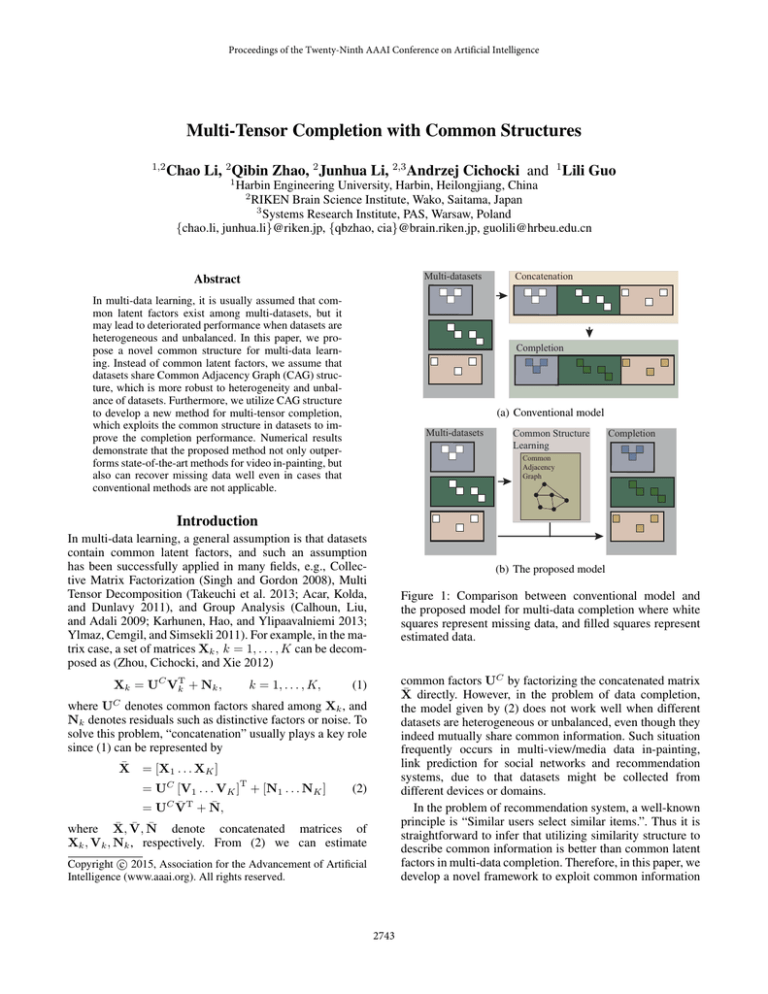
Figure 1: Comparison between conventional model and
the proposed model for multi-data completion where white
squares represent missing data, and filled squares represent
estimated data.
common factors UC by factorizing the concatenated matrix
X̄ directly. However, in the problem of data completion,
the model given by (2) does not work well when different
datasets are heterogeneous or unbalanced, even though they
indeed mutually share common information. Such situation
frequently occurs in multi-view/media data in-painting,
link prediction for social networks and recommendation
systems, due to that datasets might be collected from
different devices or domains.
In the problem of recommendation system, a well-known
principle is “Similar users select similar items.”. Thus it is
straightforward to infer that utilizing similarity structure to
describe common information is better than common latent
factors in multi-data completion. Therefore, in this paper, we
develop a novel framework to exploit common information
(1)
where UC denotes common factors shared among Xk , and
Nk denotes residuals such as distinctive factors or noise. To
solve this problem, “concatenation” usually plays a key role
since (1) can be represented by
X̄
= [X1 . . . XK ]
T
= UC [V1 . . . VK ] + [N1 . . . NK ]
(2)
= UC V̄T + N̄,
where X̄, V̄, N̄ denote concatenated matrices of
Xk , Vk , Nk , respectively. From (2) we can estimate
c 2015, Association for the Advancement of Artificial
Copyright Intelligence (www.aaai.org). All rights reserved.
2743
N k
Xk (j, l) /Nk . It can be
and μk,j is given by μk,j = l=1
found from (4) that W is actually an average correlation matrix among Xk ∈ RI×Nk , k = 1, . . . , K, and its element
W (i, j) ∈ [−1, 1] describes similarity between two entities.
If we restrict the measure to be non-negative, an alternative
measure is defined by
among datasets. Instead of common latent factors, we assume that datasets share Common Adjacency Graph (CAG)
structure (see Fig. 1). In addition, we propose a new method
for multi-tensor completion by taking the common structure
into account.
Basic model
Common adjacency graph
Wg (i, j) =
CAG
projection
...
For clarity, we first introduce the new model in the matrix
case, and then apply it for tensor data in the next subsection. Suppose that we have K matrices Xk ∈ RI×Nk , k =
1, . . . , K, and let the first mode be the common mode, i.e.
rows of matrices Xk have common structure information,
and each row of datasets is defined as an entity. Let G denote a graph in which nodes represent entities and edges represent relationships between every pair of entities in datasets
(see Fig. 2). Furthermore, a weight is assigned to each edge
to quantify how ‘close’ of entities. We call such a graph as
Common Adjacency Graph (CAG) since it can reflect the
common neighbour relationships among entities of datasets.
Xk (i, :) − Xk (j, :) 22 /Nk
Kσ
,
(5)
i, j = 1, . . . , I,
where σ denotes a tuning parameter to control the degree of
attenuation. To avoid scale diversity of datasets, we can also
use a normalized version of (5) in which we force entities to
be zero mean and unit variance. Note that W (i, j) ∈ (0, 1]
in (5) can be considered as a non-linear version of (4), and
the values are kept being always positive.
Formulas (3)-(5) represent three possible measures to describe relationships of entities. According to specific applications, we can easily extend any existing similarity measure to the model. In this paper, we only use the normalized version of (5) in experiments since it generally provides
good performance in physical data like video in-painting.
For other kinds of data, e.g., ratings and links, extensions
of Jaccard similarity and cosine similarity (Shepitsen et al.
2008) are expected to achieve satisfactory results.
entities
...
...
Dataset 1
exp −
K
k=1
Dataset K
Figure 2: Schematic diagram illustrating how matrices have
CAG structure.
More specifically, we use an adjacency matrix W ∈ RI×I
to describe weights of edges in the graph G. The i, jth element of W, denoted by W (i, j), presents the similarity between ith and jth entities. In the simplest case, we can specify W by binary values according to a priori knowledge, that
is
1
if node i and j are connected
Wp (i, j) =
. (3)
0
otherwise
Multi-tensor completion with common structures
In the problem of tensor completion, low rank approximation is usually applied to estimate missing values. Many
methods minimize the nuclear norm of a tensor since nuclear
norm is well known as the tightest convex envelope of rank
of a matrix (Fazel 2002), and has been directly extended into
tensor by (Gandy, Recht, and Yamada 2011). In the case
of multi-tensor completion, we also follow this idea, but it
should be noted that only minimizing the nuclear norm of
each individual tensor may break the structure of Common
Adjacency Graph. Thus, in the following, we will introduce
a novel multi-tensor completion method, in which not only
low rank approximation but also CAG structure is imposed
to estimate missing values in multi-tensor.
An alike manner was proposed by (Chen, Hsu, and Liao
2013), in which smoothness was imposed for single image
in-painting by a so-called differential matrix. However, such
a priori knowledge cannot be obtained in advance for most
applications. In order to learn CAG structure from data directly, one straightforward data-driven measure can be defined by
Wc (i, j) =
1
K
K
k=1
Xk (i, :) − μk,i , Xk (j, :) − μk,j ,
Xk (i, :) − μk,i 2 Xk (j, :) − μk,j 2
Suppose we have K tensors Xk , k = 1, . . . , K with
missing values that are indexed by binary tensors Bk (0unobserved, 1-observed) whose size is same to Xk . Furthermore, suppose that there is one common mode for all tensors, and datasets have CAG structure along the common
mode. Additionally we suppose the dimension of the common mode is equal to M , and let a vector c ∈ RK×1 describe the order of the common mode in each tensor. Then
the fully reconstructed tensor Yk , k = 1, . . . , K can be ob-
(4)
i, j = 1, . . . I,
where ·, · denotes inner product of two vectors, · 2
denotes Euclidean norm of a vector, Xk (i, :) , k =
1, . . . , K, i = 1, . . . , I represents the ith row of matrix Xk ,
2744
where Zk,qk has the same size to the corresponding unfold(q )
ing matrix Yk k . To search the stationary point of (7), we
update Zk,qk , Yk , ∀k, qk and W sequentially. For each matrix and tensor, we update Zk,qk , ∀k, qk by PGD methods
which has been discussed by (Cai, Candès, and Shen 2010;
Toh and Yun 2010), and update Yk and W by standard gradient methods. Pseudo-code of the algorithm is shown in
Alg.1.
tained by minimizing the following cost function
min f ({Yk |∀k} , W) =
(c(k))
(c(k))
W (i, j) Yk
(i, :) − Yk
(j, :) 22
k,i,j=i
+
λk Yk ∗
(6)
k
s.t.
P Bk (Yk ) = P Bk (Xk )
Algorithm 1 Multi-tensor completion with common structures
Input: Observation Xk and index tensors Bk , the order of
common mode c for Xk and tuning parameter λk,qk >
0, k = 1, . . . , K, qk = 1, . . . , Qk .
Output: Estimated tensors Yk
.
1: Initialize Y 0k by P Bk Y 0k = P Bk (Xk ), and fill unobserved elements by zero, compute W0 over Y0k , and
let iteration counter t = 0.
2: repeat
3:
t = t + 1.
(c(k)),t−1
4:
Zt−1
, ∀k,
k,c(k) ← RYk
where entries of R are given by
W satisfies one of (3)-(5) over Yk , ∀k
(c(k))
where c (k) denotes the kth element of vector c, Yk
denotes unfolding of tensor Yk along the c (k)th order (Cichocki et al. 2009), and W ∈ RM ×M . Yk ∗
denotes nuclear norm of Yk , which is defined
by
(q)
(q)
Yk ∗ = q,i αq · σi Yk / j αj , where σi Yk
(q)
denotes the ith singular value of Yk and αq , q = 1, . . . , Qk
represents any positive number that was set as 1 for simplicity. P Bk (·) indicates that we choose observed elements of
which the corresponding elements in Bk are equal to 1, and
λk > 0 are tuning parameters. From (6), we can find that
matrix W builds a relationship among all datasets. In other
words, it means that estimated tensors Yk have common
neighbour (i.e., CAG) structure along the common mode.
Meanwhile, we also minimize nuclear norm of individual
tensors as penalty terms to achieve low rank approximation
of observations. It is worth noting that, if let W equal a identity matrix, (6) degenerates to estimating the low rank approximation of each dataset individually. It means, in such
case no common information is utilized, but in practice there
would be more or less common information which can be
exploited to achieve better performance for multi-data analysis. If there are more than one common mode, (6) can
be straightforwardly extended by imposing additional CAG
structures.
R (i, i) = 0, i = 1, . . . , M,
R (i, j) = Wt−1 (i, j) /
Wt−1 (i, m) , i = j
m=i
5:
6:
7:
8:
9:
10:
qk ,t−1
Zt−1
, ∀k, qk = c (k)
k,qk ← Yk
t−1
, ∀k, qk
Ztk,qk ← D Zk,qk | λk,qk /2
+
Ytk ← qk ten Ztk,qk /Qk , ∀k
P Bk Ytk ← P Bk (Xk ) , ∀k
Compute Wt over Ytk , ∀k.
until convergence
Algorithm
Note that it is difficult to optimize (6) directly due to the
existence of tensor nuclear norm and the additional constraints. In order to search the optimal solution of (6) efficiently, we relax the cost function by introducing auxiliary matrices Zk,qk ∀k, qk which can be seen as an estima(q )
tion for the unfolding Yk k of tensor Yk , and the relaxed
cost function can be easily solved by Proximal Gradient
Descent (PGD) and Alternating Update (AU) methods. Let
Xk , k = 1, . . . , K be K Qk th order tensors, then a relaxation of (6) can be formulated as
min f ({Yk |∀k} , {Zk,qk |∀k, qk } , W)
W (i, j) Zk,c(k) (i, :) − Zk,c(k) (j, :) 22
=
In Alg.1, steps 4-6 are performed according to PGD,
where step 4 is derived by computing partial derivative of
(qk )
(7) w.r.t. Zt−1
= Zk,qk , ∀k, qk .
k,c(k) under the constraint Yk
Matrix R denotes a intermediate matrix in order to compact
expression, and D (·|·)+ denotes soft-thresholding the singular values of the matrix with a scalar to achieve a low rank
approximation. If X = UΣVT is the Singular Value Decomposition (SVD) of X, then D (X|λ)+ = UΣ̄VT , where
any element Σ̄ (i, j) of Σ̄ satisfies
Σ̄ (i, j) =
k,i,j=i
+
λk,qk Zk,qk ∗
Σ (i, j) − λ
0
Σ (i, j) > λ
.
otherwise
(8)
Note that ten (·) denotes folding a matrix into a tensor which
can be considered as an reverse procedure to tensor unfolding. It should be noted from Alg.1 that auxiliary variables
Zk,qk can provide closed-form solutions for each iteration,
additionally reduce mutual influence among unfolding matrices of tensors when computing tensor nuclear norm.
(7)
k,qk
(q )
s.t. P Bk (Yk ) = P Bk (Xk ) , Yk k = Zk,qk
W satisfies one of (3)-(5) over Yk , ∀k, qk
2745
are original tensors and Yk are the corresponding estimations.) of missing values and lost frame estimation in different missing percentage.
Related works
The problem of a single tensor completion has been extensively discussed in (Liu et al. 2013; Signoretto et al. 2014;
Xu et al. 2013; Zhao, Zhang, and Cichocki 2014; Acar et al.
2011), where (Zhao, Zhang, and Cichocki 2014; Acar et al.
2011) are based on tensor decomposition to achieve a low
rank approximation for completion, while (Liu et al. 2013;
Signoretto et al. 2014; Xu et al. 2013) minimize nuclear
norm of a tensor directly. However, all these methods only
focus on one single tensor (e.g., images and videos), thus
they cannot sufficiently exploit common information in the
case of multi-data task. In the case of multiple datasets,
(Singh and Gordon 2008; Bouchard, Yin, and Guo 2013;
Klami, Bouchard, and Tripathi 2013) discuss multi-matrix
completion in recommendation system, and (London et al.
2013; Nickel 2013; Nickel and Tresp 2013) developed methods for multi-relational learning. However, all these methods
hold a basic assumption that common latent factors are contained by datasets. It has been discussed previously that such
an assumption is often not sufficient in many applications.
In machine learning, (Niyogi 2004) and later (Shu, Ma, and
Latecki 2014; He, Cai, and Niyogi 2005) discussed methods
to find a locality preserving subspace for feature extraction
and classification/clustering. Inspiring by these works, we
find that CAG is an inherent structure to share common information in multiple datasets.
Table 1: RSE of estimation of multi-view videos in-painting
in different missing percentages
Methods
Proposed
MTC
FaLRTC
HardC
TMac
CPWOPT
80%
50%
Miss
Lost
Miss
Lost
Miss
Lost
0.25
0.29
0.27
0.31
0.31
0.27
0.25
0.77
N/A
N/A
N/A
N/A
0.18
0.25
0.20
0.22
0.29
0.24
0.19
0.79
N/A
N/A
N/A
N/A
0.12
0.14
0.12
0.13
0.28
0.21
0.13
0.91
N/A
N/A
N/A
N/A
For comparison, FaLRTC (Liu et al. 2013), HardC (Signoretto et al. 2014), TMac (Xu et al. 2013), and CPWOPT
(Acar et al. 2011) was individually implemented on every
video since all these methods only focused on one single tensor. Additionally, MTC (Li, Guo, and Cichocki 2014) represents a “common factor” based method which was implemented on the three videos, and the key point of MTC is
to concatenate all datasets along the common mode. It is
shown from Tab. 1 that the proposed method outperforms
other methods. For lost frame estimation, only MTC and the
proposed method work, but the performance of MTC for lost
frame estimation is seriously poor. Fig. 3 shows prediction
of two frames chosen from the first video, where the first
row represents a frame with missing pixels and the second
row represents the lost frame. Fig. 4 shows comparison of
average runtime in different missing percentage. It is shown
from Fig. 3, 4 that the proposed method can recover the lost
frames well, and its runtime is comparable to other methods.
Experimental results
Multi-view video in-painting with one frame lost
In computer vision and graphics, many methods were developed for image and video in-painting (Liu et al. 2013;
Xu et al. 2013; Zhao, Zhang, and Cichocki 2014). In our
paper, we extend in-painting problem to multi-view videos.
Furthermore, we intend to reconstruct severely damaged
videos in which not only pixels but a whole frame is lost.
In this case, numerical experiments show that conventional
methods can not satisfactorily recover the lost frame, but our
method can estimate not only missing pixels but also the
lost frame efficiently by utilizing the CAG structure among
datasets.
Specifically, in Experiment 1, we utilized multi-view
videos (Height×Width×Channel×Time) of human action
(body movement by a lady) recorded by 3 cameras simultaneously1 . Since the three videos were recorded at the same
time from different views, it is straightforward to infer that
datasets are mutually related along the time mode (i.e., common mode). Furthermore, in order to validate our method in
the case of unbalanced datasets, the three videos were resized. This unbalanced situation is always happened in real
applications due to videos are possibly recorded by different devices. For performance evaluation, we independently
run the experiment 20 times, and randomly removed some
pixels from the three videos with specific missing percentage, and randomly removed one frame from the first video
in
shows Related Square Error (RSE =
each run. Tab.1
2
2
X
−
Y
/
k
k
k
k Xk , where Xk , k = 1, . . . , K
1
90%
Video in-painting with audio information
In multi-media analysis, not only videos but also audio are
usually recorded into a multi-media file. Thus one question
arises whether we can in-paint a video in serious damaged
cases by using auxiliary information from audio or not? The
answer is obvious, but the biggest challenge is that video
and audio data are heterogeneous and extremely unbalanced.
In Experiment 2, we demonstrate that the proposed method
can recover videos with numerous frames lost ( randomly
or consecutively ) by exploiting common structures of audio
data.
In Experiment 2, a video we used was that a train passed
by a camera with sound of whistles and noise generated by
wheels, etc.2 . We extracted video and audio dataset from the
original file individually, and organize data into a tensor and
matrix respectively. For the video, the tensor was organized
as V ∈ R61×88×3×227 (Height×Width×Channel×Time).
For audio, we only choose one channel and cut it up into
227 segments which correspond to frames of the video. As
2
http://media.au.tsinghua.edu.cn/index.jsp
2746
http://v.youku.com/v show/id XNDI3NTAxMjIw.html
Proposed
method
MTC
Missing
Observed
frame
Typical
frame
Lost
Original
frame
Audio
segment
TMac
CPWOPT
Missing
HardC
Typical
frame
Lost
FaLRTC
Audio
segment
Figure 3: Performance comparisons among methods when
missing percentage of pixel was equal to 50%.
1500
Time (s)
90%
80%
Missing Percentage
The third stage
The fourth stage
it is easy to understand that they share common information
along the time mode. Fig. 6 shows adjacency matrices of
unfolding of V and A along the time mode by using (5),
where warm colors represent two entities are similar while
cool colors represent they are different from each other. It
can be easily found from Fig. 6 that both the two adjacency
matrices have some common structures to reflect different
stages of the video, which indicates that our assumption is
reasonable for video in-painting via audio information.
500
0
The second stage
Figure 5: Typical frames and corresponding audio segments
for each stage of the data in Experiment 2.
Proposed method
MTC
FaLRTC
HardC
TMac
CPWOPT
1000
The first stage
50%
Figure 4: Comparison of average run time for various methods.
(a) video data
preprocessing, we applied Fourier transform on each segment with Hamming window to obtain spectral amplitude,
and removed high frequency components since important
audio information only focused on low frequency. Finally,
we obtained the audio data as a matrix A ∈ R227×701 .
The content of the whole video can be mainly divided into
four stages. In the first stage, camera was recording the background, the train didn’t pass by the camera yet, and there is
only noise in audio; In the second stage, a yellow railway
engine passed by the camera with whistle; In the third stage,
a series of red carriages passed by the camera with the sound
of clicks of the train; The final stage was also the background
like the first stage but the corresponding sound was still click
sounds since the train was not far away from the camera.
Fig. 5 shows typical frames and their corresponding audio
segments at each stage.
Since the video and audio were recorded at the same time,
(b) audio data
Figure 6: Adjacency matrix of video and audio data for Experiment 2.
In the experiment, we first randomly removed 50% pixels of each frame from V, and randomly removed eight
frames from four stages of V. We implemented the proposed
method to recover the damaged video tensor with audio matrix A. Fig. 7 shows estimations of lost frames by the proposed method.
It is evident from Fig. 7 that the proposed method can
provide rough but reasonable estimations for lost frames by
using CAG structure shared by video and audio data. Some
details (e.g., the gate of the carriage and the 227th frame)
cannot be exactly recovered. It is because video data has totally lost this information and common information from A
2747
10th frame
30th frame
60th frame
100th frame
150th frame
180th frame
200th frame
227th frame
Lost
frame
Recovered
frame
Lost
frame
(a) Original frames
Recovered
frame
Figure 7: Recovery of lost frames by using audio information.
cannot exactly reflect details of V. For example, the 227th
frame represents that the train has passed by the camera, but
the sound of clicks of the train was still recorded by audio
since the train was still near to the camera. Therefore our
method can only infer from the audio that the train was still
passing by the camera during the 227th frame. However, it
is worth noting that our method sufficiently exploits the relationship between video and audio data to provide a fairish
estimation, while conventional methods entirely fail in this
case, which has been shown in Experiment 1.
(b) Estimations
Figure 8: Recovery of consecutive lost frames by using audio information.
Conclusion
One would argue that, since lost frames can be estimated
by imposing a priori knowledge about correlation along time
domain during completion, what is the main advantage for
the proposed method? It should be noted that the proposed
method does NOT impose any priori knowledge about video
in-painting, while we only exploit some useful information from multi-observations. We believe that the proposed
method can work for many different applications, e.g. Recommendation System and Link Prediction, as long as multidatasets share common information.
In this paper, we proposed a novel framework to exploit
common structure existing in heterogeneous datasets for tensor completion, and such a new idea breaks the conventional
assumption that multi-datasets should contain common latent factors. We developed a new structure called Common
Adjacency Graph to describe the shared information existing in multiple datasets, regardless of whether datasets are
heterogeneous or not. By using Common Adjacency Graph,
a novel multi-tensor completion method was introduced, and
results of numerical experiments show that the proposed
method outperforms conventional tensor completion methods, and can successfully reconstruct videos in the case that
conventional methods entirely fail.
Compared to the previous experiments in which lost
frames were discretely chosen, subsequently, we removed
blocks of frames from V, and applied the proposed method
for in-painting. Similarly, we first randomly removed 50%
pixels of each frames from V, but next removed consecutive
10 frames (it will last 1 sec in the video for each block) from
the first and third stages of V, respectively. Fig. 8 shows two
blocks of lost consecutive frames and their estimations by
the proposed method. It is shown in Fig. 8 that the proposed
method can estimate lost consecutive frames reliably. Since
details of lost frames of V cannot be exactly reflected from
audio data A, the estimation for lost consecutive frames is
not very high-quality. However, the result shown in Fig. 8
indicates that common information contained by audio can
be exploited for video in-painting problem, even if video and
audio data is heterogeneous and extremely unbalanced.
Acknowledgements
The authors would like to thank the reviewers for their positive feedback and constructive comments. This work was
supported by the National Natural Science Foundation of
China (Grant No. 61271263, 61401115, 61202155).
References
Acar, E.; Dunlavy, D. M.; Kolda, T. G.; and Mrup, M. 2011.
Scalable tensor factorizations for incomplete data. Chemometrics and Intelligent Laboratory Systems 106(1):41–56.
2748
Acar, E.; Kolda, T. G.; and Dunlavy, D. M. 2011. All-at-once
optimization for coupled matrix and tensor factorizations.
arXiv preprint arXiv:1105.3422.
Bouchard, G.; Yin, D.; and Guo, S. 2013. Convex collective matrix factorization. Proceedings of the Sixteenth International Conference on Artificial Intelligence and Statistics
144–152.
Cai, J.-F.; Candès, E. J.; and Shen, Z. 2010. A singular
value thresholding algorithm for matrix completion. SIAM
Journal on Optimization 20(4):1956–1982.
Calhoun, V. D.; Liu, J.; and Adali, T. 2009. A review of
group ICA for fMRI data and ICA for joint inference of
imaging, genetic, and ERP data. Neuroimage 45(1):S163–
S172.
Chen, Y.; Hsu, C.; and Liao, H. 2013. Simultaneous tensor
decomposition and completion using factor priors. Pattern
Analysis and Machine Intelligence, IEEE Transactions on
36(3):577–591.
Cichocki, A.; Zdunek, R.; Phan, A. H.; and Amari, S.-i.
2009. Nonnegative matrix and tensor factorizations: applications to exploratory multi-way data analysis and blind
source separation. John Wiley and Sons.
Fazel, M. 2002. Matrix rank minimization with applications.
Ph.D. Dissertation, PhD thesis, Stanford University.
Gandy, S.; Recht, B.; and Yamada, I. 2011. Tensor completion and low-n-rank tensor recovery via convex optimization. Inverse Problems 27(2):025010.
He, X.; Cai, D.; and Niyogi, P. 2005. Tensor subspace analysis. In Advances in neural information processing systems,
499–506.
Karhunen, J.; Hao, T.; and Ylipaavalniemi, J. 2013. Finding dependent and independent components from related
data sets: A generalized canonical correlation analysis based
method. Neurocomputing 113(0):153–167.
Klami, A.; Bouchard, G.; and Tripathi, A. 2013. Groupsparse embeddings in collective matrix factorization. arXiv
preprint arXiv:1312.5921.
Li, C.; Guo, L.; and Cichocki, A. 2014. Multi-tensor completion for estimating missing values in video data. arXiv
preprint arXiv:1409.0347.
Liu, J.; Musialski, P.; Wonka, P.; and Ye, J. 2013. Tensor
completion for estimating missing values in visual data. Pattern Analysis and Machine Intelligence, IEEE Transactions
on 35(1):208–220.
London, B.; Rekatsinas, T.; Huang, B.; and Getoor, L. 2013.
Multi-relational learning using weighted tensor decomposition with modular loss. arXiv preprint arXiv:1303.1733.
Nickel, M., and Tresp, V. 2013. Logistic tensor factorization
for multi-relational data. arXiv preprint arXiv:1306.2084.
Nickel, M. 2013. Tensor factorization for relational learning. Ph.D. Dissertation, Ludwig Maximilian University.
Niyogi, X. 2004. Locality preserving projections. In Neural
information processing systems, volume 16, 153–161.
Shepitsen, A.; Gemmell, J.; Mobasher, B.; and Burke, R.
2008. Personalized recommendation in social tagging sys-
tems using hierarchical clustering. In Proceedings of the
2008 ACM conference on Recommender systems, 259–266.
ACM.
Shu, L.; Ma, T.; and Latecki, L. J. 2014. Locality preserving
projection for domain adaptation with multi-objective learning. AAAI.
Signoretto, M.; Dinh, Q. T.; De Lathauwer, L.; and Suykens,
J. A. 2014. Learning with tensors: A framework based on
convex optimization and spectral regularization. Machine
Learning 94(3):303–351.
Singh, A. P., and Gordon, G. J. 2008. Relational learning via
collective matrix factorization. Proceedings of the 14th ACM
SIGKDD international conference on Knowledge discovery
and data mining 650–658.
Takeuchi, K.; Tomioka, R.; Ishiguro, K.; Kimura, A.; and
Sawada, H. 2013. Non-negative multiple tensor factorization. In Proc. IEEE International Conference on Data Mining (ICDM13).
Toh, K.-C., and Yun, S. 2010. An accelerated proximal
gradient algorithm for nuclear norm regularized linear least
squares problems. Pacific Journal of Optimization 6(615640):15.
Xu, Y.; Hao, R.; Yin, W.; and Su, Z. 2013. Parallel matrix
factorization for low-rank tensor completion. arXiv preprint
arXiv:1312.1254.
Ylmaz, Y. K.; Cemgil, A. T.; and Simsekli, U. 2011. Generalised coupled tensor factorisation. In Advances in Neural
Information Processing Systems, 2151–2159.
Zhao, Q.; Zhang, L.; and Cichocki, A. 2014. Bayesian CP
factorization of incomplete tensors with automatic rank determination. arXiv preprint arXiv:1401.6497.
Zhou, G.; Cichocki, A.; and Xie, S. 2012. Common and
individual features analysis: Beyond canonical correlation
analysis. arXiv preprint arXiv:1212.3913.
2749