Proceedings of the Thirtieth AAAI Conference on Artificial Intelligence (AAAI-16)
Semi-Supervised Multinomial Naive Bayes for Text Classification
by Leveraging Word-Level Statistical Constraint
Li Zhao, Minlie Huang, Ziyu Yao, Rongwei Su*, Yingying Jiang*, Xiaoyan Zhu
State Key Lab. of Intelligent Technology and Systems
Tsinghua National Laboratory for Information Science and Technology
Dept. of Computer Science and Technology, Tsinghua University, Beijing 100084, PR China
*Samsung R&D Institute China - Beijing
zhaoli19881113@126.com aihuang@tsinghua.edu.cn
+
fied as either positive or negative. Let Nloves
represent how
−
for
many times “loves” occurs in positive documents, Nloves
+
negative documents. ploves represents the probability that
word “loves” appears in positive documents, and can be es+
+
−
/(Nloves
+ Nloves
). In general, we use pcw
timated by Nloves
to represent the class distribution on word.
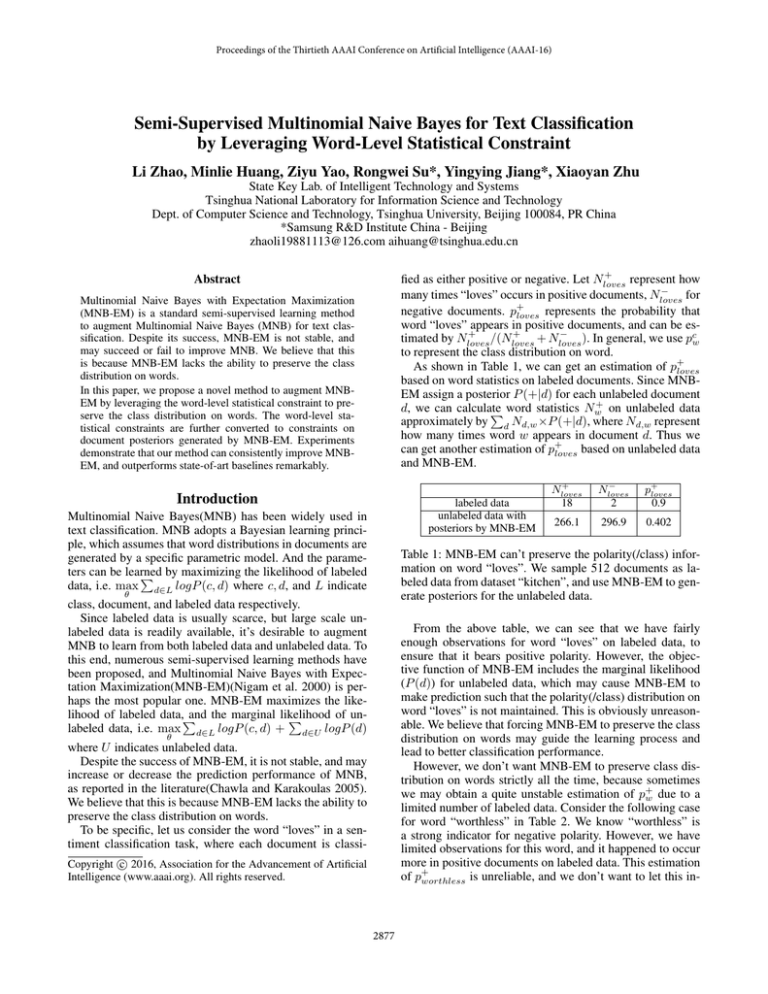
As shown in Table 1, we can get an estimation of p+
loves
based on word statistics on labeled documents. Since MNBEM assign a posterior P (+|d) for each unlabeled document
+
d, we can calculate
word statistics Nw on unlabeled data
approximately by d Nd,w ×P (+|d), where Nd,w represent
how many times word w appears in document d. Thus we
can get another estimation of p+
loves based on unlabeled data
and MNB-EM.
Abstract
Multinomial Naive Bayes with Expectation Maximization
(MNB-EM) is a standard semi-supervised learning method
to augment Multinomial Naive Bayes (MNB) for text classification. Despite its success, MNB-EM is not stable, and
may succeed or fail to improve MNB. We believe that this
is because MNB-EM lacks the ability to preserve the class
distribution on words.
In this paper, we propose a novel method to augment MNBEM by leveraging the word-level statistical constraint to preserve the class distribution on words. The word-level statistical constraints are further converted to constraints on
document posteriors generated by MNB-EM. Experiments
demonstrate that our method can consistently improve MNBEM, and outperforms state-of-art baselines remarkably.
Introduction
labeled data
unlabeled data with
posteriors by MNB-EM
Multinomial Naive Bayes(MNB) has been widely used in
text classification. MNB adopts a Bayesian learning principle, which assumes that word distributions in documents are
generated by a specific parametric model. And the parameters can be learned
by maximizing the likelihood of labeled
data, i.e. max d∈L logP (c, d) where c, d, and L indicate
+
Nloves
18
−
Nloves
2
p+
loves
0.9
266.1
296.9
0.402
Table 1: MNB-EM can’t preserve the polarity(/class) information on word “loves”. We sample 512 documents as labeled data from dataset “kitchen”, and use MNB-EM to generate posteriors for the unlabeled data.
θ
class, document, and labeled data respectively.
Since labeled data is usually scarce, but large scale unlabeled data is readily available, it’s desirable to augment
MNB to learn from both labeled data and unlabeled data. To
this end, numerous semi-supervised learning methods have
been proposed, and Multinomial Naive Bayes with Expectation Maximization(MNB-EM)(Nigam et al. 2000) is perhaps the most popular one. MNB-EM maximizes the likelihood of labeled data,
and the marginal likelihood
of un
labeled data, i.e. max d∈L logP (c, d) + d∈U logP (d)
From the above table, we can see that we have fairly
enough observations for word “loves” on labeled data, to
ensure that it bears positive polarity. However, the objective function of MNB-EM includes the marginal likelihood
(P (d)) for unlabeled data, which may cause MNB-EM to
make prediction such that the polarity(/class) distribution on
word “loves” is not maintained. This is obviously unreasonable. We believe that forcing MNB-EM to preserve the class
distribution on words may guide the learning process and
lead to better classification performance.
However, we don’t want MNB-EM to preserve class distribution on words strictly all the time, because sometimes
we may obtain a quite unstable estimation of p+
w due to a
limited number of labeled data. Consider the following case
for word “worthless” in Table 2. We know “worthless” is
a strong indicator for negative polarity. However, we have
limited observations for this word, and it happened to occur
more in positive documents on labeled data. This estimation
of p+
worthless is unreliable, and we don’t want to let this in-
θ
where U indicates unlabeled data.
Despite the success of MNB-EM, it is not stable, and may
increase or decrease the prediction performance of MNB,
as reported in the literature(Chawla and Karakoulas 2005).
We believe that this is because MNB-EM lacks the ability to
preserve the class distribution on words.
To be specific, let us consider the word “loves” in a sentiment classification task, where each document is classic 2016, Association for the Advancement of Artificial
Copyright Intelligence (www.aaai.org). All rights reserved.
2877
Additionally, we have Nw represents how many times
word w appears in labeled data. (Nw )u represents how many
times word w appears in unlabeled data. Nwc represents how
many times word w appears in documents that belong to
class c on labeled data. Nd,w , Nw , (Nw )u and Nwc are important word statistics used in our word-level statistical constraint.
formation mislead the learning process.
labeled data
unlabeled data
with posteriors
by MNB-EM
+
Nworthless
−
Nworthless
p+
worthless
7.26
15.74
0.316
2
1
0.66
Table 2: We don’t want to preserve the class information
on word “worthless” because it’s unreliable. We sample 512
documents as labeled data from dataset “kitchen”, and use
MNB-EM to generate posteriors for the unlabeled data.
MNB and MNB-EM
Multinomial Naive Bayes (MNB) addresses the task of text
classification from a Bayesian principle. MNB makes a simple assumption that word occurrences are conditionally independent of each other given the class of the document.
In order to preserve the class distribution on words in a
robust, reasonable way, we propose to use the interval estimation of pcw on labeled data, to bound the point estimation of pcw on unlabeled data. Thus our model can automatically generate tighter bounds for more frequent words, and
looser bounds for less frequent words. Those word-level statistical constraints are further converted into constraints on
document posteriors, and are injected into MNB-EM under
the framework of Posterior Regularization(PR)(Graca et al.
2007).
Our contributions are listed as follows:
• We propose a novel semi-supervised model, Multinomial Naive Bayes with Word-level Statistical
Constraint(MNB-WSC) to augment MNB-EM by
preserving class distribution on words.
• We propose a novel idea to preserve the class distribution
on words robustly : using the interval estimation of pcw
on labeled data, to bound the point estimation of pcw on
unlabeled data.
• Experiments demonstrate that our model outperforms
baselines remarkably.
The rest of this paper is organized as follows. We introduce the problem definition in Section 2. MNB and MNBEM is summarized in Section 3. In Section 4, we introduce
our word-level statistical constraint. We present our MNBWSC model in Section 5. We present experiment results in
Section 6. In Section 7, we survey related work. We summarize our work in Section 8.
P (c|d) =
P (c)
|V |
P (wi |c)Nd,wi
P (d)
i=1
(1)
MNB estimates the parameters θ = {P (wi |c), P (c)} by
maximizing the joint log likelihood of labeled data.
max
θ
logP (c, d)
(2)
d∈L
In order to leverage both labeled data and unlabeled data,
MNB-EM tries to maximize both joint likelihood of labeled
data, and marginal likelihood of unlabeled data as shown in
Eq.3
max
θ
d∈L
logP (c, d) +
logP (d)
(3)
d∈U
From the above equations, we have the following observations: 1. MNB and MNB-EM only leverages label information from the perspective of documents, i.e. P (c|d),
P (c, d), P (d). 2. MNB-EM combine labeled data and unlabeled data, by maximizing the sum of joint likelihood of
labeled data and marginal likelihood of unlabeled data to get
a point estimation for parameter.
The difference between our model and MNB-EM is twofold: First, we introduce word class distribution pcw to leverage label information from the perspective of words. Second, we combine labeled data and unlabeled data, by using
the interval estimation of pcw generated from labeled data, to
bound the point estimation of pcw generated from unlabeled
data.
Problem Definition
We focus on a semi-supervised text classification task,
which aims at assigning a correct class label c for each document d. We adopt the bag-of-words representation for documents. The set of unique words w appearing in the whole
document collection is called vocabulary V. The set of class
label c is the output space C.
Let Nd,w represents how many times word w appears
in document d. Thus document d can be represented by d
={Nd,w1 , Nd,w2 ,..., Nd,w|V | }.
We assume the following inputs:
• A set of labeled documents L = {(di , c)|i = 1, ..., |L|},
drawn i.i.d from a distribution P (d, c) .
• A large set of unlabeled documents U = {di |i = |L| +
1, ..., |L|+|U
|}, drawn i.i.d from the marginal distribution
P (d) = c P (d, c) .
Word-level Statistical Constraint
In this section, we present our data-driven constraint model.
First, we present constraint based on word class distribution
pcw , which captures how likely word w is occurring in a document that belongs to class c. Then, we show how to convert
this constraint into document posterior constraint.
Word-level Statistical Constraint
Let us consider a certain word w. In a labeled dataset, w may
occur in several documents for several times. For each time,
the document that w occurs in could belongs to any class.
So each occurrence of w can be seen as a trial, where the
document that w occurs in belongs to class c with probability pcw . We introduce a random variable Xw to denote the
2878
class of the document that contains w. We adopt the 1-of-k
representation here for Xw as follow,
1
2
k
Xw = (Xw
, Xw
, ..., Xw
)
“loves”
“worthless”
c
pcw Xw
Document Posterior Constraint
(5)
Up to now, we already get a confidence interval
[lower(pcw ), upper(pcw )] for pcw . We can apply this constraint on (pcw )u .
(6)
lower(pcw ) ≤ (pcw )u ≤ upper(pcw )
c
Or in short,
Xw ∼ M ultinomial(pw )
Given labeled data, we can estimate parameter pcw . The Maximum Likelihood Estimation(MLE) of pcw based on labeled
data is
c
N
(pcw )l = w i
i Nw
=
Nd,w × P (c|d)
d∈U Nd,w
d∈U
c
lower(pw ) × (Nw )u ≤
CI =
z2
α/2
2Nw
± zα/2
c
Nd,w × P (c|d) ≤ upper(pw ) × (Nw )u (11)
d∈U
(7)
Thus, we convert the constraint on word-statistics into constraint on document posteriors. Our constraints are datadriven constraints, which combine labeled information on
word-level from labeled data, and large-scale unlabeled data.
For each word w, we have above constraint on all the documents that contain w. Although for certain w, the constraint
could be very loose. Since we have thousands of words in
total, these constraints can still play an important role in the
learning process.
Multinomial Naive Bayes with Word-level
Statistical Constraint
In this section, we present our probabilistic model,
Multinomial Naive Bayes with Word-level Statistical
Constraint(MNB-WSC), which combines MNB-EM with
our word-level statistical constraint. Since our word-level
constraints can be converted to constraints on document posteriors, we formulate our problem in the framework of Posterior Regularization (PR)(Graca et al. 2007).
PR is an efficient framework to inject constraints on the
posteriors of latent variables. In this work, we apply PR
in the context of MNB-EM for text classification. As mentioned above, MNB-EM attempts to maximize the following
objective function.
(8)
Although labeled data can’t give us a reliable point estimation (pcw )l , it can still give us a reliable interval estimation.
We can conduct interval parameter estimation for pcw with
limited observations, and thus get a confidence interval(CI)
for pcw . We are confident that pcw is in the confidence interval. If (pcw )u , the parameter learned by MNB-EM, is a good
estimation, we are confident that (pcw )u should be in that
confidence interval, too. Because Wilson interval has good
properties even for a small number of trials and an extreme
probability,, we use Wilson interval to calculate the confidence interval for pcw here, as follows,
(pcw )l +
(10)
Substituting equation 8 into equation 10, we have
However, for large and sparse feature spaces common in settings like text classification, many words/features occur in
only a small fraction of examples, which leads to noisy and
unreliable estimation of parameter pcw .
If we estimate the parameter pcw on the classification result of MNB-EM on unlabeled data, we will get another estimation result (pcw )u , as shown in Eq.8. It’s very likely that
(pcw )u is different from (pcw )l . Since (pcw )l is noisy and unreliable for most features, it’s OK for (pcw )u being different
from (pcw )l . But the real question here, is how much could
(pcw )u be different from (pcw )l ?
(pcw )u
CI(p+
w)
[0.6990,0.9721]
[0.2076,0.9385]
Table 3: Interval estimation for word “loves” and “worthless” on labeled data. Confidence interval(CI) is calculated
at confidence level 95%.
where Xwi ∈ {0, 1}, i=1 Xwi = 1. Xwc = 1 means that
the document contains w belongs to class c. Obviously, the
class of document that w occurs in for each time follows
multinomial distribution.
Nw−
2
1
(4)
k
P r(Xw ) =
Nw+
18
2
log Lθ (D) =
logP (c, d) +
d∈L
logP (d)
(12)
d∈U
PR makes the assumption that the labeled data we have is not
enough for learning good model parameters, but we have a
set of constraints on the posterior distribution of the labels.
In our case, we can define the set of desirable posterior distributions Q according to Eq. 11 as
2
[(pcw )l (1 − (pcw )l ) + zα/2
/4Nw ]/Nw
2
(1 + zα/2
/Nw )
(9)
where we look for z-table to find zα/2 corresponding to
a certain confidence level(1 − α). By leveraging interval estimation, we can give tighter bound for more frequent words, and looser bound for less frequent words.
As shown in Table 3, we can apply interval estimation for
word “loves” and “worthless”. Word “worthless” has interval [0.2076, 0.9385], which is a loose bound and allows
the probability that “worthless” may indicate negative sentiment. We can also find that frequent words(such as “loves”)
have tighter bound.
Q = {q(c|d)|
c
Nd,w × q(c|d) ≤ upper(pw ) × (Nw )u ,
d∈U
c
Nd,w × q(c|d) ≥ lower(pw ) × (Nw )u }
(13)
d∈U
Instead of restricting pθ directly, which might not be feasible, PR penalizes the distance of pθ to the constraint set Q.
The posterior-regularized objective is termed as follows:
max{log Lθ (D) − min KL(q(C|D)||pθ (C|D))}
θ
2879
q∈Q
(14)
Evaluation Metrics
By trading off the objective function of MNB-EM (as defined in the first term), and the KL divergence of the posteriors to the valid posterior subspace defined by constraint (as
defined in the second term), the objective encourages models
with both desired posterior distribution and data likelihood.
In essence, the model attempts to maximize objective function of MNB-EM subject (softly) to the constraints.
The objective can be optimized by an EM-like scheme
that iteratively solves the minimization problem and the
maximization problem. This algorithm can be easily implemented as described in(Graca et al. 2007), so we omit it here.
We use Macro-F1 to evaluate both topic classification and
sentiment classification.
Baselines and Settings
We compare our methods with several state-of-art baselines. Below, we detail the comparison methods that we reimplemented for our experiments.
MNB Classical Multinomial Naive Bayes classifier that
only uses labeled data, “add-1” smoothing is employed here.
Experiment
Data Sets and Evaluation Metrics
MNB-EM Multinomial Naive Bayes with Expectation
Maximization(Nigam et al. 2000). We find that 15 iterations
of EM is sufficient to ensure approximate convergence to
obtain reliable parameters. The weight of an unlabeled example is set to be 1/5 the weight of a labeled example.
We evaluate on two text classification tasks: topic classification and sentiment classification.
Dataset For topic classification, we use 4 multi-class
datasets. “Ohscal” is a dataset of medical documents in
WEKA1 . “Reuters”(Rose, Stevenson, and Whitehead 2002)
is a collection of news articles organized into topics, and we
use the 8 most frequent topics here2 . WebKB(Craven et al.
1998) consists of 4,199 university webpages of four types:
course, faculty, project and student3 . 20 Newsgroups(Lang
1995) is a set of 18,828 Usenet messages from 20 different online discussion groups 4 . For sentiment classification, we use 4 domains from the Multi-Domain Sentiment
Dataset5 (Blitzer, Dredze, and Pereira 2007). Table 4 provides a brief description of each dataset.
All datasets have been widely used in previous studies,
and are publicly available. “Ohscal” is already preprocessed
by the original authors. We preprocess other datasets for
topic classification in a similar way as (Su, Shirab, and
Matwin 2011), converting to lower case characters, and
then applying tokenization, stemming, and punctuation and
stop word removal. We preprocess Multi-Domain Sentiment
Dataset in a similiar way as (Lucas and Downey 2013), since
punctuation could indicate strong sentiment.
Dataset
Ohscal
Reuters
WebKB
20News
Kitchen
Electronics
Toys&Games
Dvd
#Class
10
8
4
20
2
2
2
2
#Instance
11,162
7,674
4,199
18,828
19,856
23,009
13,147
124,438
Positive(%)
79.25
78.06
80.46
85.87
SFE Semi-supervised Frequency Estimate(Su, Shirab,
and Matwin 2011). SFE use equality P (+|w) =
Pl (+, w)/Pu (w) to estimate parameters. “Add-1” smoothing is also used in SFE.
MNB-FM MNB with Feature Marginals (Lucas and
Downey 2013). MNB-FM use feature marginals as constraints to estimate parameters for binary text classification.
Our method shares the same settings with MNB-EM. The
confidence level is set to be 80% for all dataset.
Classification Performance
We experiment with different sizes of labeled set by setting
|Tl | = {64, 128, 256, 512}. For each data set and each size,
we repeat experiments 50 times, and each time randomly
sample labeled data for training and testing. Each time, we
ensure that there is at least one document for each class.
The primary results of our experiments are shown in Table 5-6. We use one-tailed t-tests with a 95% confidence interval, to judge whether a method is significantly worse or
better than MNB-WSC.
We can see that MNB-WSC can improve MNB-EM consistently, and outperforms other state-of-art methods for
most cases. Additionally, we discuss the experiment results
from the following three perspectives: improvement against
MNB-EM, the effect of labeled data size, and performance
under imbalanced class distribution.
|V |
11,466
17,387
7,770
24,122
10,442
12,299
8,448
56,713
Improvement against MNB-EM MNB-WSC can consistently improve MNB-EM on all datasets. This is not surprising, since our method aims at solving the issues existing in
MNB-EM.
The improvement of MNB-WSC is affected by two factors: 1. How many meaningful constraints we can generate
from labeled data. 2. How bad MNB-EM is in terms of preserving word polarity. With more labeled data, and worse
performance of MNB-EM, our method can give more improvement.
Table 4: Data Description.
1
Available at http://www.cs.waikato.ac.nz/ml/weka/
Available at http://www.daviddlewis.com/resources/
testcollections/reuters21578/
3
Available at http://www.cs.cmu.edu/ WebKB/
4
Available at http://qwone.com/ jason/20Newsgroups/
5
Available at http://www.cs.jhu.edu/ mdredze/datasets/
sentiment/
2
2880
Impact of Labeled Data Size We want to compare different methods, to see how the performance changes with the
growth of labeled data size. Let us consider the performance
dataset
Kitc.
Elec.
T&G
Dvd
dataset
Kitc.
Elec.
T&G
Dvd
dataset
Kitc.
Elec.
T&G
Dvd
dataset
Kitc.
Elec.
T&G
Dvd
dataset
Ohscal
Reuters
WebKB
20News
dataset
Ohscal
Reuters
WebKB
20News
dataset
Ohscal
Reuters
WebKB
20News
MNB-WSC
0.6681
0.6627
0.6844
0.5714
MNB-WSC
0.6955
0.6947
0.7156
0.5796
MNB-WSC
0.7182
0.7212
0.7340
0.6172
Estimation of Word Class Distribution
of different methods on dataset “Ohscal”, as shown in Fig.1.
We find that: 1. MNB-EM and MNB-WSC perform especially well when labeled data size is small. 2. MNB-WSC
grows faster than MNB-EM, since with more labeled data,
we can generate more reliable constraints to guide the learning process.
number of labeled documents Tl = 64
MNB
MNB-EM
SFE
0.4644•
0.5353
0.4591•
0.4824•
0.4905
0.5330
0.6589•
0.6674
0.6911
0.3177•
0.4242
0.3204•
number of labeled documents Tl = 128
MNB
MNB-EM
SFE
0.5456•
0.5878
0.5435•
0.5843•
0.5938
0.6102
0.7157•
0.7250
0.7332
0.4115•
0.5322
0.4302•
number of labeled documents Tl = 256
MNB
MNB-EM
SFE
0.5955•
0.6166•
0.5956•
0.6789
0.6826
0.6862
0.7526
0.7425
0.7637
0.5161•
0.6175
0.5443•
number of labeled documents Tl = 512
MNB
MNB-EM
SFE
0.6420•
0.6404•
0.6399•
0.7647
0.7714
0.7656
0.7768
0.7641
0.7844
0.6235•
0.7019
0.6395•
MNB-WSC
0.6417
0.6374
0.6446
0.5546
Table 6: Comparison of Macro-F1 for Sentiment Classification. • worse, or ◦ better, comparing to MNB-WSC
Figure 1: Impact of labeled data size. Macro-F1 on data
“Ohscal”, at |Tl | = {64, 128, 256, 512}.
dataset
Ohscal
Reuters
WebKB
20News
number of labeled documents Tl = 64
MNB
MNB-EM
SFE
MNB-FM
0.5960•
0.5759•
0.6185
0.6040
0.5905•
0.5606•
0.6129
0.6099
0.5907•
0.5225•
0.6182
0.6135
0.5329
0.4827•
0.5482
0.5135
number of labeled documents Tl = 128
MNB
MNB-EM
SFE
MNB-FM
0.6185•
0.5940•
0.6405
0.6308
0.6117•
0.5829•
0.6346
0.6231•
0.6217•
0.5897•
0.6473•
0.6330•
0.5259•
0.4880•
0.5607
0.5193•
number of labeled documents Tl = 256
MNB
MNB-EM
SFE
MNB-FM
0.6431•
0.6001•
0.6639•
0.6528•
0.6412•
0.5859•
0.6602•
0.6498•
0.6618•
0.6766
0.6726•
0.6533•
0.5518
0.4937•
0.5787
0.5413•
number of labeled documents Tl = 512
MNB
MNB-EM
SFE
MNB-FM
0.6777•
0.6158•
0.6904•
0.6787•
0.6798•
0.5989•
0.6918•
0.6841•
0.6856•
0.7036•
0.6940•
0.6817•
0.5694•
0.5050•
0.6009
0.5554•
In this section, we want to evaluate how different learning
methods learn good estimation of word class distribution.
We test on “Kitchen” by setting |Tl | = 64. Table 7 shows
how word class distribution is preserved by MNB-WSC,
compared to MNB-EM. We estimate word class distribu−
tion p+
w , pw on the classification result of MNB, MNB-EM,
and MNB-WSC respectively. Then, we compute the KLdivergence of the above distribution from the true distribution over the entire data set. The average reduction of KLdivergence against MNB and MNB-EM is calculated with
respect to words with different probability and Unknown,
Half-Known, Known words. Known indicates words occurring in both positive and negative training examples, Half
Known indicates words occurring in only positive or negative training examples, while Unknown indicates words that
never occur in labeled examples. The KL-divergence from
the true distribution for MNB-WSC is smaller than the estimated distribution for MNB and MNB-EM on average.
Since MNB does not have word class distribution drift issue, our model is not strictly better than MNB on word class
distribution estimation. The overall improvement can only
imply that our model can classify documents more correctly.
MNB-WSC
0.5417
0.5359
0.6945
0.4429
MNB-WSC
0.6022
0.6291
0.7439
0.5327
MNB-WSC
0.6418
0.7054
0.7677
0.6215
MNB-WSC
0.6736
0.7723
0.7839
0.7049
Impact of Parameter
Table 5: Comparison of Macro-F1 for Topic Classification.
• worse, or ◦ better, comparing to MNB-WSC
We vary the confidence level(CL) from 70% to 95% to see
how it impacts on the performance of MNB-WSC. We test
on “Ohscal” by setting |Tl | = 512. The results are presented
in Fig. 2 . We can see that the performance is fairly stable
when changing the confidence level, which implies the robustness of our model. The robustness partially comes from
that, we apply constraints softly, instead of hardly, on the
objective function.
Performance under Imbalanced Class Distribution
From Table 6, we can see MNB-WSC outperforms all methods on all datasets under imbalanced class distribution.
This is because that our method has the potential ability
to preserve class distribution on unlabeled data, while other
methods are likely to classify all instances as the largest
class. Since our method can preserve the class distribution
on words, and many frequent words appear in most documents. Constraints on those words can preserve the class
distribution of unlabeled data.
Related Work
Semi-supervised text classification is an active research
area. However, most existing works leverages both la-
2881
Word Prop.
0-10−6
10−6 -10−5
10−5 -10−4
10−4 -10−3
> 10−3
Avg Improvement v.s. MNB
Known Half-Known Unknown
-0.0658
-0.0607
0.1919
0.0162
-0.0753
0.0427
0.0686
0.0289
0.0579
0.0695
-0.0123
-
Avg Improvement v.s. MNB-EM
Known Half-Known Unknown
0.1339
0.2206
0.0210
0.1474
0.1795
0.0902
0.0867
0.0926
0.0449
0.0618
0.3101
-
Known
0.03%
2.92%
20.67%
-
Probability Mass
Half-Known Unknown
0.02%
2.11%
1.30%
15.92%
16.45%
23.25%
12.81%
1.09%
-
−
Table 7: Analysis of {p+
w ,pw } estimation improvement of MNB-WSC over MNB and MNB-EM(Dataset “Kitchen”, |Tl | =
{64}). Known indicates words occurring in both positive and negative training examples, Half Known indicates words occurring
in only positive or negative training examples, while Unknown indicates words that never occur in labeled examples.
features that are strong indicators of certain class, while our
model can leverage all words by providing an general constraint paradigm.
Our work is also related to general constraint-driven (or
knowledge-driven) learning models, including Constraintdriven learning(Chang, Ratinov, and Roth 2007), Posterior
regularization (Graca et al. 2007), Generalized expectation
criteria (Druck 2011) and Measurements(Liang, Jordan, and
Klein 2009).
The most similar two works are (Su, Shirab, and Matwin
2011) and (Lucas and Downey 2013) in terms of augmenting MNB in a semi-supervised manner. SFE(Su, Shirab, and
Matwin 2011) re-estimates parameters by leveraging word
posteriors from labeled data and word frequency from unlabeled data. MNB-FM attempts to improve MNB’s estimation using word statistics from unlabeled data. However,
we find that SFE leverages all word posteriors directly, including those are unreliable due to limited observations.
And MNB-FM is limited to binary classification. While our
model can leverage class information on words robustly to
solve multi-class text classification problem.
To the best of our knowledge, MNB-WSC is the first approach that leverages labeled data from the perspective of
words and generate reasonable, intuitive constraints for both
frequent and less frequent words based on word statistics to
improve a semi-supervised classifier.
Figure 2: Impact of confidence level. Macro-F1 on dataset
“Ohscal” at |Tl | = 512.
beled data and unlabeled data from the perspective of
documents. Current popular Semi-Supervised Learning approaches include using Expectation-Maximization on probabilistic models (Nigam et al. 2000); Transductive Support
Vector Machines (Joachims 1999); and graph-based methods(Zhu and Ghahramani 2002)(Lin and Cohen 2011)(Liu,
He, and Chang 2010)(Subramanya and Bilmes 2009). Compared with these works, our model can also leverages labeled
data from the perspective of words.
Another line of works focus on unsupervised text classification by leveraging “labeled feature”. Labeled feature
refers to the feature that is a strong indicator of certain
class. For example, in a baseball vs. hockey text classification problem, even without any labeled data, we know that
the presence of the word puck is a strong indicator of hockey.
Labeled feature is human-provided domain knowledge. Several works have explored labeled feature by Generalized
Expectation Criteria(GEC) (Mann and McCallum 2007),
by Non-negative Matrix Tri-factorization(NMF)(Li, Zhang,
and Sindhwani 2009), by document-word co-regularization
on bipartite graph(Sindhwani and Melville 2008), by combining both labeled feature and labeled document(Melville,
Gryc, and Lawrence 2009).
Our work is similar to works on labeled feature in terms
of both leveraging the labeled information from the perspective of words. The key difference here is two-fold:1. Labeled
feature is human-provided knowledge, while our word-level
statistic constraint is data-driven constraint generated from
labeled data. 2. Works on labeled feature only leverage those
Conclusion
In this paper, we propose a novel semi-supervised learning method to augment MNB-EM by leveraging the wordlevel statistical constraint to preserve the class distribution
on words. Experiments show that our method can consistently improve the performance of MNB-EM, and outperforms state-of-art baselines. We also show that out methods
can produce more accurate estimation of word class distribution.
We also propose a novel idea to combine information
from two views, in our case, labeled data and unlabeled
data. Traditional methods usually adopt an objective function that is the sum of the objective function from each view.
We propose to use interval estimation of certain parameter
from one view(in our case, labeled data), to bound the point
estimation of the parameter from another view(in our case,
unlabeled document posteriors provided by MNB-EM). We
believe this idea is interesting and intuitive, and has potential impact on many learning problems. We will try to apply
2882
this idea to other learning problems in our future work.
26th Annual International Conference on Machine Learning, ICML ’09, 641–648. New York, NY, USA: ACM.
Lin, F., and Cohen, W. W. 2011. Adaptation of graph-based
semi-supervised methods to large-scale text data.
Liu, W.; He, J.; and Chang, S.-F. 2010. Large graph
construction for scalable semi-supervised learning. In
Fürnkranz, J., and Joachims, T., eds., Proceedings of
the 27th International Conference on Machine Learning
(ICML-10), 679–686. Haifa, Israel: Omnipress.
Lucas, M., and Downey, D. 2013. Scaling semi-supervised
naive bayes with feature marginals. In ACL (1), 343–351.
The Association for Computer Linguistics.
Mann, G. S., and McCallum, A. 2007. Simple, robust,
scalable semi-supervised learning via expectation regularization. In Proceedings of the 24th International Conference
on Machine Learning, ICML ’07, 593–600. New York, NY,
USA: ACM.
Melville, P.; Gryc, W.; and Lawrence, R. D. 2009. Sentiment
analysis of blogs by combining lexical knowledge with text
classification. In Proceedings of the 15th ACM SIGKDD International Conference on Knowledge Discovery and Data
Mining, KDD ’09, 1275–1284. New York, NY, USA: ACM.
Nigam, K.; McCallum, A. K.; Thrun, S.; and Mitchell, T.
2000. Text classification from labeled and unlabeled documents using em. Mach. Learn. 39(2-3):103–134.
Rose, T.; Stevenson, M.; and Whitehead, M. 2002. The
reuters corpus volume 1 - from yesterday’s news to tomorrow’s language resources. In Proceedings of the Third International Conference on Language Resources and Evaluation, 329–350.
Sindhwani, V., and Melville, P. 2008. Document-word coregularization for semi-supervised sentiment analysis. In
ICDM, 1025–1030. IEEE Computer Society.
Su, J.; Shirab, J. S.; and Matwin, S. 2011. Large scale
text classification using semisupervised multinomial naive
bayes. In Getoor, L., and Scheffer, T., eds., ICML, 97–104.
Omnipress.
Subramanya, A., and Bilmes, J. A. 2009. Entropic graph
regularization in non-parametric semi-supervised classification. In Bengio, Y.; Schuurmans, D.; Lafferty, J. D.;
Williams, C. K. I.; and Culotta, A., eds., NIPS, 1803–1811.
Curran Associates, Inc.
Zhu, X., and Ghahramani, Z. 2002. Learning from labeled
and unlabeled data with label propagation. Technical report.
Acknowledgement
This work was partly supported by the National Basic Research Program (973 Program) under grant
No.2012CB316301 /2013CB329403, the National Science
Foundation of China under grant No.61272227/61332007,
and the Beijing Higher Education Young Elite Teacher
Project. The work was also supported by Tsinghua University Beijing Samsung Telecom R&D Center Joint
Laboratory for Intelligent Media Computing.
References
Blitzer, J.; Dredze, M.; and Pereira, F. 2007. Biographies,
bollywood, boomboxes and blenders: Domain adaptation for
sentiment classification. In In ACL, 187–205.
Chang, M.-W.; Ratinov, L.-A.; and Roth, D. 2007. Guiding
semi-supervision with constraint-driven learning. In Carroll,
J. A.; van den Bosch, A.; and Zaenen, A., eds., ACL. The
Association for Computational Linguistics.
Chawla, N. V., and Karakoulas, G. 2005. Learning from
labeled and unlabeled data: An empirical study across techniques and domains. J. Artif. Int. Res. 23(1):331–366.
Craven, M.; DiPasquo, D.; Freitag, D.; McCallum, A.;
Mitchell, T.; Nigam, K.; and Slattery, S. 1998. Learning
to extract symbolic knowledge from the world wide web. In
Proceedings of the Fifteenth National/Tenth Conference on
Artificial Intelligence/Innovative Applications of Artificial
Intelligence, AAAI ’98/IAAI ’98, 509–516. Menlo Park,
CA, USA: American Association for Artificial Intelligence.
Druck, G. 2011. Generalized Expectation Criteria for
Lightly Supervised Learning. Ph.D. Dissertation, University
of Massachusetts Amherst.
Graca, J. V.; Inesc-id, L.; Ganchev, K.; Taskar, B.; Graa,
J. V.; Inesc-id, L. F.; Ganchev, K.; and Taskar, B. 2007.
Expectation maximization and posterior constraints. In In
Advances in NIPS, 569–576.
Joachims, T. 1999. Transductive inference for text classification using support vector machines. In Proceedings of
the Sixteenth International Conference on Machine Learning, ICML ’99, 200–209. San Francisco, CA, USA: Morgan
Kaufmann Publishers Inc.
Lang, K. 1995. Newsweeder: Learning to filter netnews. In
in Proceedings of the 12th International Machine Learning
Conference (ML95.
Li, T.; Zhang, Y.; and Sindhwani, V. 2009. A non-negative
matrix tri-factorization approach to sentiment classification
with lexical prior knowledge. In Proceedings of the Joint
Conference of the 47th Annual Meeting of the ACL and
the 4th International Joint Conference on Natural Language
Processing of the AFNLP: Volume 1 - Volume 1, ACL ’09,
244–252. Stroudsburg, PA, USA: Association for Computational Linguistics.
Liang, P.; Jordan, M. I.; and Klein, D. 2009. Learning from
measurements in exponential families. In Proceedings of the
2883