Proceedings of the Thirtieth AAAI Conference on Artificial Intelligence (AAAI-16)
Discrete Image Hashing Using
Large Weakly Annotated Photo Collections
Hanwang Zhang† , Na Zhao† , Xindi Shang† , Huanbo Luan‡ , Tat-seng Chua†
†
National University of Singapore
‡
Tsinghua University
†
hanwang,zhaona,shangxin,chuats@comp.nus.edu.sg, ‡ luanhuanbo@gmail.com
Abstract
We address the problem of image hashing by learning binary codes from large and weakly supervised
photo collections. Due to the explosive growth of usergenerated media on the Web, this problem is becoming critical for large-scale visual applications like image
retrieval. While most existing hashing methods fail to
address this challenge well, our method shows promising improvement due to the following two key advantages. First, we formulate a novel hashing objective
that can effectively mine implicit weak supervision by
collaborative filtering. Second, we propose a discrete
hashing algorithm, offered with efficient optimization,
to overcome the inferior optimizations in obtaining binary codes from real-valued solutions. In this way, our
method can be considered as a weakly-supervised discrete hashing framework which jointly learns image semantics and their corresponding binary codes. Through
training on one million weakly annotated images, our
experimental results demonstrate that image retrieval
using the proposed hashing method outperforms the
other state-of-the-art ones on image and video benchmarks.
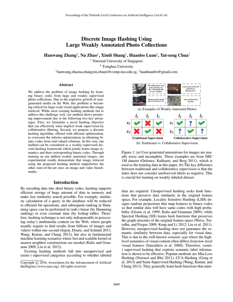
Out walking home early
in the morning, i see
this. A Macintosh Plus
in a tree.. Briljant!
2 pretty girl and the old
school bus in
Thammasart U.
Reagan in pink striped
dress in front yard - 82
some colorful fish by
the dock
(a) Examples of Weakly-Annotated Photos
l1
l2
l3
l1
x1
x1
x2
x2
Traditional Supervision
l2
l3
Collaborative Supervision
(b) Traditional vs. Collaborative Supervision
Figure 1: (a) User-generated annotations for images are usually noisy and incomplete. These examples are from SBU
1M dataset (Ordonez, Kulkarni, and Berg 2011), which is
used as the training data in this paper. (b) The key difference
between traditional and collaborative supervision is that the
latter does not consider unobserved labels as negative. This
is crucial for training on weakly-labeled dataset.
Introduction
By encoding data into short binary codes, hashing supports
efficient storage of huge amount of data in memory and
make fast similarity search possible. For example, similarity calculation of a query in the database will be reduced
to efficient bit operations, and subsequent ranking in Hamming space can be performed in (sub-) linear (by Hamming
ranking) or even constant time (by lookup table). Therefore, hashing technique is not only indispensable in processing today’s multimedia content on the Web, where people
usually require to find results from billions of images and
videos within one second (Jegou, Douze, and Schmid 2011;
Wang, Kumar, and Chang 2012), but also in fundamental
machine learning scenarios where fast and scalable kernel or
nearest neighbor constructions are needed (Kulis and Grauman 2009; Liu et al. 2012).
Existing hashing methods fall into unsupervised and
(semi-) supervised categories according to whether labeled
data are required. Unsupervised hashing seeks hash functions that preserve data similarity in the original feature
space. For example, Locality Sensitive Hashing (LSH) designs random projections that map features to binary codes
so that similar data will have same codes with high probability (Gionis et al. 1999; Kulis and Grauman 2009); while
Spectral Hashing (SH) learns hash functions that preserves
the graph structure of the original feature space (Weiss, Torralba, and Fergus 2009; Kong and Li 2012; Liu et al. 2011).
However, unsupervised hashing does not guarantee the semantic similarity between data, especially for visual data.
This is due to the well-known semantic gap where the highlevel semantics of visual content often differs from low-level
visual features (Smeulders et al. 2000). Therefore, (semi) supervised hashing that exploits semantic label information is shown to be effective. Popular methods are Min-Loss
Hashing (Norouzi and Blei 2011), CCA-Hashing (Gong et
al. 2013) and Semi-Supervised Hashing (Wang, Kumar, and
Chang 2012). They generally learn hash functions that mini-
c 2016, Association for the Advancement of Artificial
Copyright Intelligence (www.aaai.org). All rights reserved.
3669
high portion of missing annotations by efficient sparse matrix factorizations, and CF naturally supports multi-labeled
training images. We develop a formulation that alternatively
optimizes the binary codes that involve CF and quantization loss. For solution, we propose a discrete optimization
method which directly learns the binary codes and the corresponding hash functions. Thus, the quantization loss is theoretically guaranteed to be minimized without any relaxation.
Our algorithm only requires simple matrix multiplications
and inversion of small matrices, and thus can be efficiently
applied in large-scale settings. To demonstrate the effectiveness of the proposed method, we train our model on a lM
Flickr photo collection with over 30K number of weak labels and test its performance in retrieval on two challenging image and video benchmarks. Experimental results show
promising improvement over other state-of-the-art hashing
methods.
mize pair-wise similar/dissimilar Hamming distance cost according to labeling supervision. Supervised hashing requires
sufficiently large training data to achieve good generalizations for new samples. However, obtaining high-quality labeled data is usually prohibitively expensive in practice.
In recent years, with the surge in popularity of social networks, users have generated almost inexhaustible multimedia contents with weak annotations such as Flickr (see Figure 1(a)). Therefore, it is interesting to investigate whether
such large amount of weakly labeled collection can help in
learning image hash codes. In particular, we aim to tackle
the following challenges that few existing supervised hashing techniques address:
• Quantization Loss. The discrete constraints imposed on
binary code learning lead to NP-hard mixed-integer programming (Håstad 2001). Therefore, most supervised
hashing methods resort to relaxing the problem by discarding the discrete constraints, e.g., solving continuous
problem and then followed by thresholding or minimizing quantization loss (Gong et al. 2013). Although relaxation makes the original problem feasible, its resulting
hash functions are less effective due to the accumulated
quantization error. In real large-scale applications which
require longer code length for sufficient precision, the performance drop caused by quantization loss will be more
severe.
Related Work
For space limitation, we only review recent hashing methods that cover the idea of discrete optimization and multilabel supervision. For comprehensive reviews, please refer
to (Wang et al. 2014; Grauman and Fergus 2013).
The most widely used discrete hashing technique is perhaps Iterative Quantization (ITQ) (Gong et al. 2013). It minimizes the quantization loss by alternatively learning the binary codes and the hashing function. However, it has two
drawbacks. First, ITQ requires the hashing function be orthogonal projection, which is not applicable in many other
supervised objectives. Second, its optimization is a postprocessing after learning the major objective (e.g., geometry or semantic preserving similarities). Thus, ITQ is suboptimal to the objective task. Discrete Graph Hashing (Liu
et al. 2014a) and Supervised Discrete Hashing (Shen et al.
2015) are recently proposed methods based on discrete optimization. They demonstrate that jointly minimizing quantization loss and major objective function through discrete optimization can improve the hashing performance. Our work
is also an advocate of discrete optimization but focuses on
the problem of weakly supervised learning with multi-label
data. Weakly Supervised Hashing (Mu, Shen, and Yan 2010)
focuses on hashing trained by partially labeled training data,
where the definition of “weak” is more similar to “semisupervised” while we focus on “incomplete” labeling. Besides, it needs kernel and CCCP (Concave-Convex Procedure) optimization which does not scale up to large-scale
data and labels. (Gong et al. 2013) tackle multi-labeled data
as cross-modality fusion and apply CCA to obtain the correlated representation between the data and label. Then, the
representations quantize to be hashing codes by ITQ. (Zhao
et al. 2015) cast multi-label supervision into ranking supervision according to the number of shared labels. However,
these two methods cannot be applied in our weakly labeled
case since the noisy incomplete labels of data will mislead
the training. The idea of using collaborative filtering to handle weakly labeled data is similar to (Liu et al. 2014b). However, their work neglects to handle the incompleteness of
labels, which is the most essential motivation of collaborative filtering. Based on the above discussion, to our best
• Multi- vs. Single-Label. Training images collected from
social networks are multi-labeled in nature. However,
most supervised hashing methods focus on two-class pairwise relations; for multi-labeled data, the relation between
two images is no longer the simple similar/dissimilar relations, but the more complex multi-level semantic similarities. Though some works (Zhao et al. 2015; Norouzi,
Blei, and Salakhutdinov 2012) can transform the multilevel similarities into ranking objectives, they do not scale
up to large-scale training data since they require combinatorial number of ranking pairs or triplets for training.
• Weak vs. Full Supervision. As compared to full supervision, where data are fully labeled across all class labels,
weakly labeled data are generally not annotated with complete class labels. This is reasonable since casual users
are reluctant to provide complete tags. As shown in Figure 1(a), as compared to the entire English vocabulary,
annotations are generally sparse and weak. Unfortunately,
traditional supervised hashing methods strictly enforce
the missing labels as negative, and hence inevitably harm
the subsequent semantic understanding.
In this paper, by addressing the above challenges, we propose a novel hashing framework for learning hash functions
by using a large and weakly labeled photo collection. We
propose to bring Collaborative Filtering (CF), which has
been successfully applied in discovering the weak relationship between many users and items (Koren, Bell, and Volinsky 2009), to analyze the weak but abundant associations
between images and labels and then predict the new (unobserved) image-label associations (see Figure 1(b)). The
key motivation is that CF can elegantly avoid modeling the
3670
knowledge, this work is the first to learn hash functions for
large-scale, weakly labeled data with explicit discrete optimization. Thanks to the large-scale learning, the learned
hash functions can well generalize to test data even if they
are very different from training. This allows us to, say, train
on images but test on videos.
better the resulting binary codes will preserve the desired
solution in Eq. (2). Therefore, we expect that the (linear)
hash functions can minimize the quantization error:
min B − WT X2F + λW2F , s.t. B = sgn(WT X).
W
where λW2F scales the linear model W and hence scales
C. However, it is impractical to directly solve W since
sgn(·) is non-differentiable. As in ITQ (Gong et al. 2013),
we cast the problem into an iterative procedure:
Problem Formulation
We use bold upper-case letter A as matrix, bold lower-case
letter with subscript ai as the i-th column of A, and uppercase letter with subscript Aij as the entry at i-th row and j-th
column. We have n training images {x1 , x2 , ..., xn }, where
xi ∈ Rd represents the feature vector in d-dimensional
space, and a column of data matrix X ∈ Rd×n . Our goal is
to generate b hash codes B ∈ {±1}b×n for the images. The
advantage of denoting the binary codes by {±1} is that the
Hamming distance between image i and j is a strict monotonically decreasing function of the vector product bTi bj
and simplifies the formulation of learning to hash. In this
paper, we only consider linear functions,
bi = sgn(WT xi ),
min B − WT X2F + λW2F , s.t. B ∈ {±1}b×n .
W,B
2
min A − UT B A + λ1 B − WT X2F +λ2 W2F ,
U,B,W
F
Quantization
Loss
Collaborative Supervision
(1)
s.t. B ∈ {±1}b×n , UUT = I.
(5)
Note that we instantiate the regularization for U as the orthogonal constraint, which scales U and decorrelate the basis latent features of the labels as well. This objective function is not convex, we will design an iterative algorithm to
find a local optimum.
Optimization
The proposed algorithm tackles three challenges in optimizing Eq. (5): 1) the Hadamard multiplication with A; 2) the
orthogonal constraint UUT = I; and 3) the discrete constraint B ∈ {±1}b×n . We will detail our solutions in the
following three subproblems.
Collaborative Supervision and Quantization Loss
We propose to use Collaborative Filtering (CF) to effectively
uncover the semantic relations hidden in weak supervision.
In particular, we focus on the matrix factorization-based CF,
which has been demonstrated to be one of the most successful CF methods (Koren, Bell, and Volinsky 2009). Suppose
ui ∈ Rb and cj ∈ Rb are the latent vectors of label i and
image j, we expect that inner product uTi cj is large if image
j is annotated with label i, and small otherwise. Although
Collaborative Hashing (Liu et al. 2014b) is also based on this
idea, we argue that counting missing labels caused by weak
supervision as negative labels, i.e., uTi cj should be small
if Aij = 0, is not reasonable. Therefore, our collaborative
supervision model strictly stick to the definition of classic
CF (Koren, Bell, and Volinsky 2009), by only learning from
the observed annotations (i.e., Aij = 0),
U,C
(4)
As compared to the two-step methods such as ITQ which
is sub-optimal, we propose to jointly optimize the collaborative supervision objective in Eq. (2) and the quantization
loss in Eq. (4). The overall objective function is formulated
as:
where W ∈ Rd×b is the matrix of b linear hash functions
and sgn(·) is the element-wise function that sgn(x) = 1 if
x > 0 and −1 otherwise. We learn W from the labeled
data. Each image has an m-dimensional annotation (i.e., m
words), ai ∈ Rm , which is a column of label matrix A ∈
Rm×n . Note that the labels are weakly supervised, that is,
most entries of A is empty. In particular, we use Aij = 1 to
denote that image j is labeled with word i and Aij = 0 if
we have no observation on whether image j is labeled with
i. Note that it is the crucial difference from traditional multilabel supervision which considers Aij = 0 as negative.
2
min A − UT C AF + λ1 R(U) + λ2 R(C),
(3)
Fix B and U, update W This subproblem reduces to
a simple linear regression: minW λ1 B − WT X2F +
λ2 W2F , which can be solved efficiently by
W←
−1
λ2
XXT +
I
XBT .
λ1
(6)
Since (XXT + λ2 /λ1 I)−1 is fixed during optimization, we
can precompute and store its inversion for efficiency.
Fix B and W, update U By expanding the quadratic
terms according to U in Eq. (5), the subproblem of updating
U can be rewritten as:
min F (U) =
UUT =I
−
(2)
i
j∈Ii
Aij (cTj
= −tr(ABT U) +
where is the Hadamard (element-wise) matrix multiplication, which does not count the loss if Aij = 0; R(·) is any
regularization that scales the resultant U and C.
Given code bi = sgn(ci ) = sgn(WT xi ), it is easy to
show that the smaller the quantization loss bi − ci is, the
+
1
2
bTj )
i
ui +
i ui ,
uTi B
1
2
i j∈Ii
uTi bj bTj ui
(7)
where Ii denotes
the nonzero indices in the i-th row of A,
T
i = and B
j∈Ii bj bj . We apply a gradient descent with
orthogonality constraint (Wen and Yin 2013) to solve the
3671
challenging quadratic programming in Eq. (7). Suppose the
learning rate is η, the update rule at each iteration is:
UT ← UT − ηR I +
η T
L R
2
−1
LT UT ,
Algorithm 1: Discrete Weakly-Supervised Hashing
(8)
where R = [GT , UT ], L = [UT , −GT ], and G is the gra 1 u1 , ..., B
m um ]. In pracdient of F (U): G = −BAT + [B
tice, before we start the update iteration, we apply GramSchmidt process to force UUT = I since the orthogonality
constraint may deteriorate after a certain number of iterations due to numeric instability.
1
2
3
Fix U and W, update B This binary constraint in this
subproblem is generally NP-hard (Håstad 2001). Therefore,
many methods solve a relaxed problem by dropping the discrete constraint but obtain a sub-optimal result. Here, we
propose an efficient algorithm that enforces the constraint
to directly achieve discrete B.
Due to the Hadamard product of A in Eq. (5), we cannot
derive a solution for B in matrix formulation. Fortunately,
since column bj independently contributes to the loss, we
can update bj in parallel. Noting the fact that UUT = I
and bTj bj = b, the expansion of Eq. (5) according to the
j-th column of B is:
const − 2
i∈Ij
−bTj
5
6
7
8
9
10
Aij uTi
ui uTi
i∈I
/ j
4
bj + bTj UUT bj + bTj bj
constant
Algorithmic Analysis
(9)
Initialization Since the proposed formulation in Eq. (6)
is non-convex, the above optimization needs a good choice
of initial solution. Thus, we here suggest a strategy to obtain one. For initializing U and B, we solve an relaxed
minUUT =BBT =I A − UT B2F without specially dealing
with the unobserved labels. This problem can be efficiently
solved with SVD (Liu et al. 2014b) if we initialize B or U
by Gram-Schmidt process. Then, the initialization of B is
B ← sgn(B). The underlying heuristic of this initialization
is that the quantization loss minimization is meaningless unless we have already obtained a good real-valued solution of
the major objective.
bj − 2λ1 xTj Wbj ,
where Ij is the nonzero indices of the j-th column of A.
Thus, this B-subproblem reduces to maximizing the following n independent problems:
max
bj ∈{±1}b
where H =
i∈I
/ j
Input : X ∈ Rd×n : training image features,
A ∈ {0, 1}m×n : weakly-labeled annotation,
b: bit size,
η: learning rate,
λ1 and λ2 : trade-off parameter
Output: W ∈ Rd×b : linear hashing model
Initialization:
(U(0) , B∗ ) = arg minUUT =BBT =I A − UT B2F ,
B(0) = sgn(B∗ ), W(0) is random, t = 0
repeat
W-subproblem:
−1
T
W(t+1) ← XXT + λ2 /λ1 I
XB(t) ;
U-subproblem:
−1 T (t) T
T
T
U(t+1) ← U(t) − ηR I + η2 LT R
L U
according to Eq. (8);
B-subproblem (parallel updating):
for j=1 to n do (t+1)
(t)
(t)
bj
← sgn I(Hbj + p, bj
according to
Eq. (11);
end
t ← t + 1;
until converge;
return W(t)
1 T
bj Hbj + pT bj ,
2
ui uTi , pT = λ1 xTj W +
(10)
i∈Ij
Aij uTi .
We maximize the function f (b) = 12 bT Hb + pT b in
Eq. (10) iteratively. In particular, at the (t + 1)-th iteration, we maximize a surrogate function f˜t (b) = f (b(t) ) +
∇f T (b(t) )(b − b(t) ), where we denote the maximum solution as b(t+1) . Since f (b) is a convex function (H
is semi-positive definite), we have the fact f (b(t+1) ) ≥
f˜t (b(t+1) ) ≥ f˜t (b(t) ) = f (b(t) ). Therefore, we can ensure
that the sequential solution {b(t) } will iteratively converge
to a local maximum solution to Eq. (10). According to the
above analysis, we can easily derive the update rule for bj
as:
bj ← sgn(I(∇f (bj ), bj )) = sgn (I(Hbj + p, bj ) ,
Complexity In training stage, the major space consumption is the image feature matrix X which requires O(dn).
Fortunately, state-of-the-art image features are usually
sparse (Donahue et al. 2013). In our case, it requires only
3-GB memory to store 1M images. Other space consumptions including U, B, and the precomputed XXT in Eq. (6)
and G in Eq. (8) are O(bn + bm + bd), which is moderate
since d and b are small. At each training iteration, the time
consumption for W-subproblem in Line 3 Alg (1) is only
O(d2 bn) since the inversion can be computed off-line. For
U-subproblem in Line 4, it requires O(b3 + mb2 ) for b × bsize eigen-decomposition and matrix multiplications. For Bsubproblem in Line 5, it requires O(sb2 + db) for constructing H and p, where s = O(n) is the number of nonzero
entries in A. For the update rule, it requires only O(b2 ).
By parallel updating, it requires O( np (sb2 + db)) in total,
where p is number of parallel computing threads. Based on
the above analysis, we can see that the time complexity of
(11)
where I(x, y) is an element-wise function such that
I(x, y) = x if x = 0 and I(x, y) = y otherwise. The above
update rule states that the updated bj should have the same
signs as ∇f (bj ); if the derivative is zero at certain entries,
we do not update the corresponding bits.
3672
10 4
Obj. Function Value
Obj. Function Value
5
4.5
4
3.5
3
10
20
30
40
50
3
10 5
Search Protocol and Metric
2.5
We adopted Hamming ranking as our search protocol. All
the data in the database are ranked according to their Hamming distance from the query and the top ranked data are returned as the results. Another widely used protocol is Hash
lookup, where a lookup table is constructed and results are
data within a Hamming radius (e.g., 2). Although Hamming
ranking requires linear search time as compared to the constant time in Hash lookup, the former provides better quality
measurement of the learned Hamming embedding while the
latter only focuses on search speed and fails to handle the
case that the bit size is larger than 32 (Wang, Kumar, and
Chang 2012). Since our testing data are labeled, for evaluation metric, we used the popular Precision@K (K from 1 to
500) with class labels as the groundtruth (Gong et al. 2013).
2
1.5
1
0.5
10
Iteration
20
30
40
50
Iteration
(a) With Initialization
(b) W/O Initialization
Figure 2: Convergence curve of the objective function using
a sub-sampled dataset with 0.1M data, b = 32, λ1 = 1,
λ2 = 1e − 4.
our algorithm is linear to the sample size: O(T n), where T
is the number of iterations. In our experiments, we found
that we usually needed T ≤ 50 for convergence. On our Intel i7 6-core machine with 3.0Ghz CPU and 64-GB memory,
we needed about 1 hour per iteration for training 1M data.
In testing stage, we only needed to store W of the size d × b
to generate hash codes for images.
Compared Methods
We compared the proposed hashing method: Ours, against
6 state-of-the-art hashing methods:
LSH (Gionis et al. 1999): Locality Sensitive Hashing. This
method models hashing function W as a Gaussian random
matrix.
PCA-ITQ (Gong et al. 2013): this method uses W =
Wpca R, where Wpca is the PCA projection and R is a rotation matrix learned by their proposed iterative quantization.
CCA-ITQ (Gong et al. 2013): this method replaces the PCA
projection to CCA projection Wcca , which is learned from
two data modalities: the image feature X and the label A.
DGH (Liu et al. 2014a): the recently proposed Discrete
Graph Hashing. This method can be considered as an advanced version of Spectral Hashing (Weiss, Torralba, and
Fergus 2009) since it supports large-scale training data and
discrete minimization for quantization loss.
CH (Liu et al. 2014b): Collaborative Hashing. It applies collaborative filtering for training hash functions. In particular,
we modified this method by applying the collaborative supervision used in this paper. Note that the original CH neglects specially modeling the unobserved labels.
SDH (Shen et al. 2015): Supervised Discrete Hashing. It
considers data hashing codes as the features for multi-label
supervised training, through which the hashing functions
can be learned simultaneously.
Among the above methods, LSH, PCA-ITQ and DGH are
unsupervised; CCA-ITQ, CH and SDH are supervised. Although there are many other supervised hashing methods,
they were not compared since they cannot be easily extended to multi-label training data. Except LSH and CH,
the rest of them have discrete optimization. We implemented
these methods using the codes provided by the authors with
default parameters. We used L2-Baseline which performs
search using 2 -norm Euclidean distance between original
features as the baseline.
Convergence Due to space limit, we omit rigorous proof
for convergence. Generally, one can easily complete the
proof based on the fact that the proposed algorithm monotonically decreases towards the lower-bounded objective
function. We show the convergence of the algorithm in Figure 2, which implies that proper initialization is necessary.
Experiments
Dataset
For training the hashing function, we used a large weaklyannotated image dataset called SBU (Ordonez, Kulkarni,
and Berg 2011). It contains 1M images with user-generated
captions. For each image, the words of caption can be considered as the observed labels. After removing stop- and
low-frequency words, we had 30,456 labels in total, i.e., matrix A is of the size 30, 456 × 1M . In order to simulate practical search scenario, where application database is usually
different from training, we used two additional benchmarks
for testing: NUSWIDE (Chua et al. 2009) and CCV (Jiang
et al. 2011). Note that our train/test split is more challenging than traditional split which is done on the same dataset.
NUSWIDE and CCV respectively contain 269,648 images
and 9,317 videos across 81 and 20 semantic classes. Note
that the number of data in each class varies from tens to thousands. For fair comparison, queries were uniformly sampled
from each class. This gave rise to 4,860 and 3,560 queries
for NUSWIDE and CCV, respectively. For each dataset,
database was considered as the whole dataset except the
query. We sampled 10 query sets for averaging the results.
We used the advanced DeCAF deep learning visual features
for images (Donahue et al. 2013) and the feature dimension
was d = 4, 096. In particular, for each video, we sampled
1 frame image in every 5 frames and the feature vector was
the mean of all the sampled frames.
Parameter Sensitivity
We empirically set λ2 to 1e − 4 since we did not find any
performance drop around 1e − 4. As compared to λ2 , λ1 is
a more crucial trade-off parameter since it balances between
the supervised loss and the quantization loss. As in Figure 5,
3673
LSH
PCA-ITQ
CCA-ITQ
DGH
CH
SDH
0.8
0.8
0.7
0.7
0.7
0.7
0.6
0.5
0.4
100
200
300
400
0.6
0.5
0.4
500
Number of top returned images
100
200
300
400
0.6
0.5
0.4
500
Number of top returned images
(a) 32 bits
Precision
0.8
Precision
0.8
Precision
Precision
L2 Baseline
100
200
300
400
0.6
0.5
0.4
500
Number of top returned images
(b) 64 bits
Ours
100
200
300
400
500
Number of top returned images
(c) 128 bits
(d) 256 bits
Figure 3: Performance (Precision@K) of various methods with different bit sizes on NUSWIDE.
LSH
PCA-ITQ
CCA-ITQ
DGH
CH
SDH
0.6
0.6
0.5
0.5
0.5
0.4
0.3
0.2
0.4
0.3
0.2
100
200
300
400
500
Number of top returned videos
(a) 32 bits
0.4
0.3
0.2
0.1
0.1
Precision
0.6
0.5
Precision
0.6
Precision
Precision
L2 Baseline
100
200
300
400
500
Number of top returned videos
0.4
0.3
0.2
100
200
300
400
500
Number of top returned videos
(b) 64 bits
Ours
(c) 128 bits
100
200
300
400
500
Number of top returned videos
(d) 256 bits
Figure 4: Performance (Precision@K) of various methods with different bit sizes on CCV.
0.8
0.4
Figure 3 and Figure 4 illustrate the retrieval results of various methods using different bit sizes on both datasets. We
can see that our proposed method considerably outperform
the other methods, especially the recently proposed CH and
SDH. This demonstrates the effectiveness of our two main
proposals: collaborative supervision for weak labels and discrete hashing.
In this paper, we explored a novel hashing framework that
uses discrete optimization for learning large and weaklylabeled data. We argued that this is an essential but challenging task since although large training data is beneficial
for supervised hashing , it rarely works because it fails to
mean Precision
0.7
0.65
0.6
mean Precision
Results
First, on both datasets and all bit sizes, we can see that
the state-of-the-art supervised methods are generally better
than the unsupervised methods. In particular, our method
outperforms the recently proposed and competitive supervised method: SDH. Although we both approach discrete
optimization, SDH adopts the traditional supervision, which
is confused by the unobserved weak labels. This may also
explain why CCA-ITQ performs the worst among supervised methods since it directly attempts to model the explicit
correlations between image features and label vectors.
Second, as compared to CH, the reason why our method
performs much better is discrete optimization. Note that our
implementation for CH is the same as the proposed method
but without discrete optimization. This demonstrates the effectiveness of minimizing quantization loss in hashing.
Third, we can see that with longer bit size, the supervised hashing performance can even outperform L2 baseline. That is to say, through supervised training, we can
perform more accurate retrieval with much lower time and
storage cost. This demonstrates the effectiveness of supervised hashing using large training data. Note that the testing
datasets NUSWIDE and CCV differ from the training set:
SBU, therefore, our promising results on this challenging
task offers large potentials in practical hashing applications.
32 bits
64 bits
128 bits
256 bits
0.75
32 bits
64 bits
128 bits
256 bits
0.35
0.3
0.25
0.55
0.5
-3 -2.5 -2 -1.5 -1 -0.5 0 0.5 1 1.5 2 2.5 3
log 1
(a) NUSWIDE
0.2
-3 -2.5 -2 -1.5 -1 -0.5 0 0.5 1 1.5 2 2.5 3
log 1
(b) CCV
Figure 5: Mean Precision from top 1 to top 500 retrieval
results on the two datasets with various bit size and λ1 .
we plot the mean precision, averaged from top 1 to 500, of
various bit size and λ1 . We can find that our algorithm is
not very sensitive to λ1 . Therefore, in all experiments, for a
certain bit size, we set λ1 to the value with best performance.
For the learning rate η used in U-subproblem, we initially
set it to 1e − 3 and used a dynamic learning rate updating
heuristic (Qian 1999).
Conclusions
3674
resolve the noisy and sparse nature of weak supervision. We
tackled this challenge by adopting the key idea of how collaborative hashing can successfully handle weak relationships. By addressing this motivation, we developed a formulation which jointly models the collaborative supervision
and quantization loss. In particular, we proposed an efficient
algorithm that explicitly uses discrete optimization to avoid
unnecessary quantization loss during optimization. Through
training on one million weakly annotated images and testing
on two challenging benchmarks, our method considerably
outperformed various state-of-the-art hashing techniques.
Norouzi, M., and Blei, D. M. 2011. Minimal loss hashing
for compact binary codes. In ICML.
Norouzi, M.; Blei, D. M.; and Salakhutdinov, R. R. 2012.
Hamming distance metric learning. In NIPS.
Ordonez, V.; Kulkarni, G.; and Berg, T. L. 2011. Im2text:
Describing images using 1 million captioned photographs.
In NIPS.
Qian, N. 1999. On the momentum term in gradient descent
learning algorithms. Neural networks.
Shen, F.; Shen, C.; Liu, W.; and Shen, H. T. 2015. Supervised discrete hashing. arXiv preprint arXiv:1503.01557.
Smeulders, A. W.; Worring, M.; Santini, S.; Gupta, A.; and
Jain, R. 2000. Content-based image retrieval at the end of
the early years. TPAMI.
Wang, J.; Shen, H. T.; Song, J.; and Ji, J. 2014. Hashing for
similarity search: A survey. arXiv preprint arXiv:1408.2927.
Wang, J.; Kumar, S.; and Chang, S.-F. 2012. Semisupervised hashing for large-scale search. TPAMI.
Weiss, Y.; Torralba, A.; and Fergus, R. 2009. Spectral hashing. In NIPS.
Wen, Z., and Yin, W. 2013. A feasible method for optimization with orthogonality constraints. Mathematical Programming.
Zhao, F.; Huang, Y.; Wang, L.; and Tan, T. 2015. Deep
semantic ranking based hashing for multi-label image retrieval. In CVPR.
Acknowledgements
This work was supported by NUS-Tsinghua Extreme Search
(NExT) project (grant R-252-300-001-490) and the National
Natural Science Foundation of China (grant 61303075).
References
Chua, T.-S.; Tang, J.; Hong, R.; Li, H.; Luo, Z.; and Zheng,
Y. 2009. Nus-wide: a real-world web image database from
national university of singapore. In CIVR.
Donahue, J.; Jia, Y.; Vinyals, O.; Hoffman, J.; Zhang, N.;
Tzeng, E.; and Darrell, T. 2013. Decaf: A deep convolutional activation feature for generic visual recognition. arXiv
preprint arXiv:1310.1531.
Gionis, A.; Indyk, P.; Motwani, R.; et al. 1999. Similarity
search in high dimensions via hashing. In VLDB.
Gong, Y.; Lazebnik, S.; Gordo, A.; and Perronnin, F. 2013.
Iterative quantization: A procrustean approach to learning
binary codes for large-scale image retrieval. TPAMI.
Grauman, K., and Fergus, R. 2013. Learning binary hash
codes for large-scale image search. In MLCV.
Håstad, J. 2001. Some optimal inapproximability results.
JACM.
Jegou, H.; Douze, M.; and Schmid, C. 2011. Product quantization for nearest neighbor search. TPAMI.
Jiang, Y.-G.; Ye, G.; Chang, S.-F.; Ellis, D.; and Loui,
A. C. 2011. Consumer video understanding: A benchmark
database and an evaluation of human and machine performance. In ICMR.
Kong, W., and Li, W.-J. 2012. Isotropic hashing. In NIPS.
Koren, Y.; Bell, R.; and Volinsky, C. 2009. Matrix factorization techniques for recommender systems. Computer.
Kulis, B., and Grauman, K. 2009. Kernelized localitysensitive hashing for scalable image search. In CVPR.
Liu, W.; Wang, J.; Kumar, S.; and Chang, S.-F. 2011. Hashing with graphs. In ICML.
Liu, W.; Wang, J.; Ji, R.; Jiang, Y.-G.; and Chang, S.-F.
2012. Supervised hashing with kernels. In CVPR.
Liu, W.; Mu, C.; Kumar, S.; and Chang, S.-F. 2014a. Discrete graph hashing. In NIPS.
Liu, X.; He, J.; Deng, C.; and Lang, B. 2014b. Collaborative
hashing. In CVPR.
Mu, Y.; Shen, J.; and Yan, S. 2010. Weakly-supervised
hashing in kernel space. In CVPR.
3675