Proceedings of the Thirtieth AAAI Conference on Artificial Intelligence (AAAI-16)
Submodular Asymmetric Feature Selection in Cascade Object Detection
†
Baosheng Yu† and Meng Fang‡ and Dacheng Tao† and Jie Yin§
Centre for Quantum Computation and Intelligent Systems, University of Technology, Sydney
‡
Department of Computing and Information Systems, The University of Melbourne
§
CSIRO, Australia
baosheng.yu@student.uts.edu.au, meng.fang@unimelb.edu.au
dacheng.tao@uts.edu.au, jie.yin@csiro.au
2003). The cascade explicitly uses a cascade of node classifiers with increasing complexity. Each node classifier is
used to correctly reject a portion of non-object windows
(measured by false positive rate) and retain any possible object windows for further precessing (measured by detection
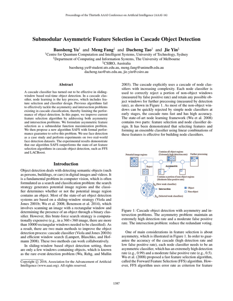
rate), as shown in Figure 1. As most of the non-object windows can be quickly rejected by simple node classifiers at
early stages, the cascade runs fast and has high accuracy.
The state-of-art node learning framework (Wu et al. 2008)
contains two parts: feature selection and node classifier design. It has been demonstrated that selecting features and
forming an ensemble classifier using linear combinations of
these features is effective for building node classifiers.
Abstract
A cascade classifier has turned out to be effective in slidingwindow based real-time object detection. In a cascade classifier, node learning is the key process, which includes feature selection and classifier design. Previous algorithms fail
to effectively tackle the asymmetry and intersection problems
existing in cascade classification, thereby limiting the performance of object detection. In this paper, we improve current
feature selection algorithm by addressing both asymmetry
and intersection problems. We formulate asymmetric feature
selection as a submodular function maximization problem.
We then propose a new algorithm SAFS with formal performance guarantee to solve this problem. We use face detection
as a case study and perform experiments on two real-world
face detection datasets. The experimental results demonstrate
that our algorithm SAFS outperforms the state-of-art feature
selection algorithms in cascade object detection, such as FFS
and LACBoost.
Introduction
Object detection deals with detecting semantic objects (such
as persons, buildings, or cars) in digital images and videos. It
is a fundamental problem in computer vision, which is often
formulated as a search and classification problem: the search
strategy generates potential image regions and the classifier determines whether or not the potential image region
contains an object. Most of the state-of-art object detection
systems are based on a sliding-window strategy (Viola and
Jones 2001b; Wu et al. 2008; Benenson et al. 2014), which
involves scanning an image with a rectangular window and
determining the presence of an object through a binary classifier. However, this brute-force search strategy is computationally expensive (e.g., in a 360×360 image, there are more
than 10000 rectangular windows needed to be classified). As
a result, there are two main methods to improve the object
detection process: cascade classifier (Viola and Jones 2001b)
and efficient window search (Lampert, Blaschko, and Hofmann 2008). These two methods can work collaboratively.
In sliding-window based object detection setting, there
are only a few windows containing objects, which is known
as the rare event detection problem (Wu, Rehg, and Mullin
Figure 1: Cascade object detection with asymmetry and intersection problems. The asymmetry problem: maintain an
extremely high detection rate and a moderate false positive
rate. The intersection problem: reduce the redundant voting.
One of main considerations in feature selection is about
asymmetry, which is illustrated in Figure 1. In order to guarantee the accuracy of the cascade (high detection rate and
low false positive rate), each node classifier needs to be an
asymmetric classifier, which has an extremely high detection
rate (e.g., 0.99) and a moderate false positive rate (e.g., 0.5).
Wu et al. (2008) proposed a fast feature selection algorithm,
called the Forward Feature Selection (FFS) algorithm. However, FFS algorithm uses error rate as criterion for feature
c 2016, Association for the Advancement of Artificial
Copyright Intelligence (www.aaai.org). All rights reserved.
1387
selection without considering the asymmetry problem. Shen
et al. (2013) also proposed a new feature selection algorithm
LACBoost, which uses a weighted error rate as criterion for
feature selection.
Another important consideration is about intersection,
which is related to the redundancy of weak classifiers
(Paisitkriangkrai, Shen, and van den Hengel 2014). Each
node classifier in the cascade is built as an ensemble by
selecting a set of weak classifiers. Each weak classifier hi
is associated with a single feature i ∈ E = {1, 2, . . . , d},
and thus it is also called a single-feature classifier 1 , which
can only correctly classify a small portion of training examples. Therefore, features need to be carefully selected in
order to guarantee the accuracy of an ensemble classifier. On
the one hand, more selected weak classifiers are expected to
reach a consensus towards classifying a given example, so
that the ensemble classifier can make a correct decision. On
the other hand, all the node classifiers should correctly classify as many training examples as possible to achieve high
coverage. There is a trade-off between improving accuracy
on each training example and improving the voting coverage
on all training examples. In other words, voting on the training examples already correctly classified is redundant and
useless. We give an intuitive example in Figure 1, where hA
indicates current selected weak classifiers hi (i ∈ A ⊂ E),
ha (a ∈ E \ A) indicates a new weak classifier based on new
chosen feature and the non-object items in the shaded region
indicates negative examples correctly classified. The new
weak classifier is useless to the examples in the intersection
area (overlapping area of two shaded regions). Therefore, it
would be desirable to select proper features that could reduce redundant votes among node classifiers. However, the
intersection problem described above has not been properly
addressed by previously proposed approaches.
In this paper, we propose a new feature selection algorithm called Submodular Asymmetric Feature Selection or
SAFS that simultaneously considers the asymmetry and intersection problems. Submodularity is an intuitive notion of
diminishing returns, which states that adding a redundant
item to a set is useless. The intersection problem addressed
in this paper can be well-captured by such a submodular
function. Inspired by this, we first reformulate feature selection as a submodular maximization problem (Krause and
Golovin 2012). We then solve it by a greedy algorithm and
provide the performance guarantee. There are three main
contributions of our work: 1) we explicitly address the intersection problem; 2) we introduce submoduarity to describe
the intersection problem in asymmetric feature selection; 3)
we proposed a new efficient algorithm to solve asymmetry
and intersection problems simultaneously.
The remainder of this paper is organized as follows. We
first briefly review the related works of cascade object detection and submodularity. We then describe the asymmetry
and intersection problems respectively. After that, we formulate the feature selection process as a submodular function maximization problem. We then propose a new algo-
rithm SAFS with performance guarantee to solve it. Lastly,
we perform experiments on two real-world face detection
datasets.
Related Work
Cascade object detection framework was firstly proposed
by Viola and Jones (2001b), which used AdaBoost to train
a node classifier. An improved variant of AdaBoost called
AsymBoost has been proposed by Viola and Jones(2001a) in
order to solve the asymmetry problem. However, both these
works need to retrain all weak classifiers at each iteration.
As a result, they are computationally prohibitive and it takes
several weeks to train the whole cascade (Viola and Jones
2004).
Recently, Wu et al. (2008) decouples the node learning
process into two parts: feature selection and ensemble classifier design. There are several works focusing on the design of ensemble classifiers, which have been demonstrated
to work well for object detection (Viola and Jones 2001a;
Wu, Mullin, and Rehg 2005; Shen et al. 2013). As an important part of node learning, feature selection has been
addressed by many studies (Wu, Rehg, and Mullin 2003;
Wu et al. 2008; Shen et al. 2013). For example, Wu et al.
(2008) proposed a fast feature selection algorithm called
FFS, which greedily selects an optimal set of features so as
to minimize error rate of the ensemble classifier. However,
FFS algorithm does not take the asymmetry problem into
consideration. Later, Shen et al. (2013) proposed an asymmetric feature selection algorithm called LACBoost, which
is based on the biased minimax probability machine (Huang
et al. 2004) and shares the same formulation with linear
asymmetric classifier (Wu et al. 2008). The LACBoost is
approximately formulated as a quadratic programming problem and entropic gradient is used to solve this problem. Similar to Adaboot, LACBoost algorithm has almost the same
computation complexity because of solving the quadratic
programming problem in each iteration. However, none of
these works have well addressed the intersection problem.
Here, our proposed algorithm considering both the asymmetry and intersection problems simultaneously.
Submodularity has turned out to be effective in solving
a lot of NP-hard problem, such as the set cover problem
(Iyer and Bilmes 2013), sensor placement (Krause, Singh,
and Guestrin 2008) and diverse recommendation (Ashkan
et al. 2014; Yue and Guestrin 2011). The intersection problem in feature selection is similar to a set cover problem, which can be well described by a submodular function. Submodularity has been used in many feature selection
as well as subset selection problems (Krause et al. 2008;
Das and Kempe 2011; Das, Dasgupta, and Kumar 2012;
Liu et al. 2013). However, these submodularity based feature selection algorithms can not be used in cascade object
detection setting, because none of them considers the asymmetry problem, which only appears in cascade object detection setting. Our work formulates the feature selection problem in cascade object detection as a submodular function
maximization problem and propose an efficient algorithm to
solve it with performance guarantee.
1
Training method of the weak classifier shows in Wu et al.
(2008)
1388
Problem Description
In Lemma 1, we know that error rate is a weighted sum
of false negative rate and false positive rate. Previously, FFS
algorithm uses error rate (or weighted error rate) as criterion
for feature selection. However, it is not equal to the node
learning goal. For the node learning goal, an extremely high
detection rate is necessary while we can always increase the
number of node classifiers to achieve a proper false positive
rate. As a result, it is more reasonable to treat false negative
rate as a constraint and then try to minimize false positive
rate under this constraint.
In this section, we first briefly introduce the cascade framework and the node learning process. We then describe the
asymmetry and intersection problems in feature selection respectively. Lastly, we formulate the problem of asymmetric
feature selection.
Node Learning
Let X = {(xi , yi )}m
i=1 be a training dataset, where xi ∈
Rd is a feature vector and yi ∈ {−1, 1} is the label of
xi . Let E = {1, 2, . . . , d} denote a set of features, P =
{(xi , yi )|(xi , yi ) ∈ X, yi = 1} denote the set of all positive
examples and N = {(xi , yi )|(xi , yi ) ∈ X, yi = −1} denote
the set of all negative examples. Let H = {H1 , H2 , . . . } denote the cascade and H ∈ H denote a node classifier. We
describe the cascade framework in Algorithm 1.
Intersection Problem
Intersection problem appears in feature selection of node
learning and we describe it as follows: in node learning
framework, each feature is corresponding to a weak classifier and each weak classifier can only correctly vote to a special set of examples. That is, given weak classifiers hi , hj ,
which can correctly vote to Xi , Xj ⊆ X, i.e., ∀(x, y) ∈
Xi , hi (x) = y and ∀(x, y) ∈ Xj , hj (x) = y. Both hi and
hj will vote to all examples (x, y) ∈ Xi ∩ Xj , thus there
may exist redundant voting. For a new chosen weak classifier ha , it will be no help to classifying examples that have
been correctly classified by hA,θ . We describe this problem
as intersection problem.
As described in asymmetry problem, we treat false negative rate as a constraint and then try to minimize false positive rate under this constraint. In other words, we try to maximize the number of negative examples correctly classified
under a constraint. For the ensemble classifier, less intersection means a more evenly voting to training examples and
reducing the redundant voting. As a result, the voting differences between negative examples and positive examples are
maximum. We can then use a threshold θ to correctly classify all positive examples and as much negative examples as
possible. We give an intuitive example in Figure 2, where
Figure 2(b) is a better voting result. More negative examples
are correctly classified in Figure 2(b) comparing to Figure
2(a) and it means lower false positive rate in Figure 2(b).
Algorithm 1 The cascade framework
Input: P, N and bootstrapping negative examples D.
Output: H = {H1 , H2 , . . . , HK } // the cascade.
1: for r = 1, 2, . . . , K do
2:
-Training node classifier Hr by P, N . // node learning.
3:
-H = H ∪ {Hr }.
4:
-Update N according to Hr and D. // bootstrapping.
5: end for
In Algorithm 1, node learning process is the key to construct a good cascade. The node learning process is decoupled into two parts: feature selection and ensemble classifier
design. For fair comparison, we use the same voting method
for the ensemble classifier (Wu et al. 2008). Let hi denote
the weak classifier corresponding to feature i ∈ E, which is
actually a single-feature classifier. Let A ⊆ E denote a set of
selected features, then the ensemble classifier corresponding
to feature set A can be constructed by the voting results of
all weak classifiers hi (i ∈ A) and a threshold θ, i.e.,
hi (x) − θ .
(1)
H(x) = hA,θ (x) = sgn
i∈A
Asymmetry Problem
The goal of node learning, which is to achieve an extremely
high detection rate and a moderate false positive rate, is
asymmetric in detection rate and false positive rate. We
demonstrate the relationship between error rate, false negative rate (= 1 − detection rate) and false positive rate in
Lemma 1.
Lemma 1. Let F P denote the false positive rate, F N denote the false negative rate and ER denote the error rate.
Then we have
Figure 2: Example of intersection problem in feature selection.
ER = α ∗ F P + (1 − α) ∗ F N,
Inspired by this, we try to select a set of features (or weak
classifiers) that maximize the number of negative examples
bellow the threshold θ. It is obvious that more negative examples below the threshold θ mean lower false positive rate
under the same detection rate constraint. Lastly, the node
where α is the proportion of negative examples in training
set.
Proof. In Appendix.
1389
For the ensemble classifier used in node learning process,
more weak classifiers will increase the accuracy of ensemble classifier and computation complexity at the same time.
Considering the computation cost, we choose a subset of
weak classifiers corresponding to feature set A (A ⊆ E
and |A| ≤ k) with maximum value f (A). Under the base
assumption that more weak classifiers will increase the accuracy of ensemble classifier, we prove that f (A) is a monotone submodular function in Theorem 1.
learning goal is equal to
P r{hA,θ (x) = −1|y = −1},
max
A,θ
P r{hA,θ (x) = 1|y = 1} ≥ 1 − β,
A ⊆ E, |A| ≤ k.
s.t.
(2)
Submodular Asymmetric Feature Selection
In this section we first formulate the feature selection process as a submodular function maximization problem by
considering both the asymmetry and intersection problems.
We then propose a greedy algorithm, which is called Submodular Asymmetric Feature Selection or SAFS, to solve
feature selection problem efficiently.
Theorem 1. f (A) = P r{hA,θA (x) = −1|y = −1} is
a monotone submodular function under a base assumption
that more weak classifiers will increase the accuracy of the
ensemble classifier.
Proof. Let hA,θA (x), hB,θB (x) denote two ensemble classifiers corresponding to feature set A ⊂ B ⊆ E. Let a ∈ E\B
denote a new feature added to the feature set A and B. We
first prove that f (A) is a monotone function and then prove
that f (A) is a submodular function.
Under the base assumption that more weak classifiers will
increase the accuracy of the ensemble classifier, we have
that: ∀(x, y) ∈ X and hA,θA (x) = y, then hB,θB (x) = y
with high probability. Let Xa = {(x, y)|ha (x) = −1, y =
−1}, XA = {(x, y)|hA,θA (x) = −1, y = −1} and
XB = {(x, y)|hB,θB (x) = −1, y = −1}. We then have
XA ⊆ XB . As a result,
Submodular Maximization
As described before, we formulate the node learning goal
as (2). However, it is a NP-hard problem, which means that
the optimal solution can not be found in polynomial time.
The intersection problem is actually same with a maximum
coverage problem or a set cover problem, which can be wellcaptured by a submodular function (Iyer and Bilmes 2013).
Inspired by this, we prove that (2) is equal to a submodular
function maximization problem.
Definition 1. (submodularity). Let E be a nonempty finite
set and 2E be a collection of all subsets of E. Let f : 2E →
R be a submodular function, i.e.,
∀X ⊆ Y ∈ 2E and a ∈ E \ Y, f (a|X) ≥ f (a|Y ),
f (B) − f (A)
= P r{hB,θB (x) = y|y = −1}
− P r{hA,θA (x) = y|y = −1}
= P r{hA,θA (x) = 1, hB,θB (x) = −1|y = −1}
|XB \ XA |
≥ 0.
=
|P |
(3)
where f (a|X) = f (X ∪ {a}) − f (X).
Definition 2. (monotonity) Let E be a nonempty finite set
and 2E be a collection of all subsets of E. Let f : 2E → R
be a monotone function, i.e.,
∀X ⊆ Y ∈ 2E , f (Y ) ≥ f (X).
(4)
That is, f (B) ≥ f (A), i.e., f (A) is a monotone function.
Next, we prove f (A) is a submodular function. Let Xa|A =
XA∪{a} \ XA and Xa|B = XB∪{a} \ XB . Then we have
Let A ⊆ E denote a subset of features and gθ (A) =
P r{hA,θ (x) = −1|y = 1}. Let fθ (A) denote the true negative rate of a node classifier, i.e.,
fθ (A) = P r{hA,θ (x) = −1|y = −1}.
(5)
f (a|A) − f (a|B)
= P r{hA,θA (x) = hA∪{a},θA∪{a} (x) = −1|y = −1}
We then rewrite (2) as follows:
max
A,θ
s.t.
− P r{hB,θB (x) = hB∪{a},θB∪{a} (x) = −1|y = −1}
fθ (A),
A ⊆ E, |A| ≤ k, gθ (A) ≤ β.
|Xa|A | − |Xa|B |
|P |
| (XB \ XA ) ∩ Xa |
=
|P |
≥ 0.
=
(6)
Considering that the node learning goal in (2) equals to
maximizing the number of negative examples below of the
threshold θ, we set θ as the maximum possible value under
the constraint gθ (A) ≤ β, i.e.,
θA =
max
θ:gθ (A)≤β
θ.
f (A) = fθA (A) = P r{hA,θA (x) = −1|y = −1}.
(8)
The feature selection problem in (9) is thus defined as a
submodular function maximization problem, i.e.,
We can then translate (6) as follows:
max f (A), s.t. |A| ≤ k.
(11)
That is, f (a|A) ≥ f (a|B), i.e., f (A) is a submodular function. From (10) and (11), we have that f (A) is a monotone
submodular function.
(7)
Thus we have
A:A⊆E
(10)
A∗ ∈ arg max f (A), s.t., |A| ≤ k.
(9)
A:A⊆E
1390
(12)
features |A∗ | = k, then for all positive integer l and |A| = l,
we have
l
l
f (A) ≥ 1 − e− k max f (A) = 1 − e− k f (A∗ ).
Algorithm
Inspired by Nemhauser, Wolsey, and Fisher (1978), we propose a new asymmetric feature selection algorithm, which is
called Submodular Asymmetric Feature Selection or SAFS.
In SAFS algorithm, we greedily choose each feature a,
which maximally increases the value of f (A ∪ {a}), i.e.,
a ∈ arg max f (A ∪ {a}).
|A|≤k
Proof. See proof of Theorem 1.5 in Krause and Golovin
(2012).
(13)
In Theorem 3, if the optimal set of features is A∗ (|A∗ | ≤
k), then we can always find a set |A| = l ≥ k by SAFS that
makes f (A) quickly converge to f (A∗ ), which is illustrated
in Figure 3.
a:a∈E\A
From (13) and the definition of f (A), SAFS algorithm
chooses the new feature according to two respects: 1) the
new ensemble classifier hA∪{a},θA∪{a} satisfies the constraint that detection rate is greater or equal to 1 − β; 2) the
new ensemble classifier maximumly increases the number of
negative examples correctly classified (i.e., maximumly reduces the false positive rate). The detail of SAFS algorithm
is shown in Algorithm 2.
1
F(β)
0.8
0.6
0.4
Algorithm 2 The SAFS algorithm
0.2
Input: X, E and k(|A| ≤ k).
Output: hA,θA // the node classifier.
1: Make a table Vi,j = hi (xj ), for all i ≤ d and j ≤ m.
2: for t = 1, 2, . . . ,k do
3:
H(x) = sgn
hi (x) − θA∪{a} .
0
0
1
2
3
β
4
5
6
Figure 3: Let β = l/k and F (β) = f (A)/f (A∗ ), then F (β)
converges to 1 very quickly.
i∈A∪{a}
4:
f (A ∪ {a}) =
m
1{H(xi ) = −1, yi = −1}.
Experiment
i=1
5:
a ∈ arg max f (A ∪ {a}).
In this section, we used face detection as a case of object detection and performed experiments on two real-world
face detection dataset. The experimental results compare our
SAFS algorithm with current state-of-art feature selection
algorithms, such as FFS and LACBoost. Also, a random selection or RS algorithm is used as a baseline in our experiments.
a:a∈E\A
6:
A = A ∪ {a}.
7: end for
8: hA,θA (x) = sgn
hi (x) − θA .
i∈A
As (12) is still a NP-hard problem, we show a 1 − 1e approximation bound for SAFS algorithm in Theorem 2.
Datasets
Theorem 2. Let f : 2 → R+ be defined in (8) and A be
the greedily selected set defined in (13). We then have
1
f (A) ≥ 1 −
max f (A).
e |A|≤k
E
We used two real-world face detection datasets in our experiments.
• CBCL Face Database #1 2 : It consists of a training set
of 6977 images (2429 face and 4548 non-face) and a test
set of 24045 images (472 face and 23573 non-face) and
all face images are aligned to a base resolution of 19 × 19
pixels.
Theorem 2 is simply derived from Nemhauser, Wolsey,
and Fisher (1978). We can then guarantee
that
the worst case
of our algorithm will not worse than 1 − 1e -approximation
of the optimal solution and it is the best result for a
polynomial-time algorithm (Nemhauser, Wolsey, and Fisher
1978). That is, if the optimal classifier (error rate = 0) uses k
features and
set is A∗ , then we can guarantee that
the feature
f (A) ≥ 1 − 1e f (A∗ ) ≈ 0.632 ( i.e., false positive rate
≤ 1 − 0.632 = 0.368), where A is selected by our SAFS
algorithm. Also, we provide an important extension of Theorem 2 according to Krause and Golovin (2012) in Theorem
3, which enhances the effectiveness of our algorithm.
• Caltech 10,000 Web Faces 3 : It contains images of people collected from the web through Google Image Search.
The dataset has 10,524 human faces of various resolutions
and in different settings, e.g. portrait images, groups of
people, etc. All faces are cropped into a base resolution of
36 × 36 pixels.
For each dataset, we used totally 2000 frontal face images.
The faces were selected by filtering away faces which are not
2
MIT Center For Biological and Computation Learning,
http://www.ai.mit.edu/projects/cbcl
3
http://www.vision.caltech.edu/Image Datasets/
Theorem 3. Let f : 2E → R+ be defined in (8) and A be
the greedily selected set defined in (13). If the optimal set of
1391
False Positive Rate.
100
200
k/ Number of features.
(a)
300
RS
FFS
LACBoost
SAFS
0.8
0.6
0
0
100
200
k/ Number of features.
(b)
100
200
300
1
RS
FFS
LACBoost
SAFS
0.8
0.2
0
0.6
300
0
0
100
200
k/ Number of features.
(c)
1
300
RS
FFS
LACBoost
SAFS
0.8
0.6
0.4
k/ Number of features.
(d)
RS
FFS
LACBoost
SAFS
0.2
0.6
0.4
1
0.8
0.4
0.2
1
0.2
0
0.6
0.4
0.2
0
0
RS
FFS
LACBoost
SAFS
False Positive Rate.
0.4
1
0.8
False Positive Rate.
0.6
False Positive Rate.
RS
FFS
LACBoost
SAFS
False Positive Rate.
False Positive Rate.
1
0.8
100
200
k/ Number of features.
(e)
0.4
0
300
100
200
k/ Number of features.
(f)
300
Figure 4: False Positive Rate of the ensemble classifiers using RS, FFS, LACBoost and SAFS algorithm.
semble classifiers on both two datasets.
1
0.99
0.98
0.98
0.97
0.96
0.95
0
False Positive Rate Measure
Detection Rate
1
0.99
Detection Rate
high enough resolution, upright, or front facing. The nonface images were sampled and cropped from 273 high resolution scene images, which were similar to Wu et al. (2008).
To train a node classifier, our training data contained 1000
frontal face images and 1000 non-face images. In each image, we used 5000 features sampled uniformly from all rectangle features similar to Wu et al. (2008), which contained
five type of Harr-like features. For testing, we used 1000
frontal face images and 1000 non-face images in our experiments.
0.5
RS
FFS
LACBoost
SAFS
1
k/ Fasle Positive Rate
0.97
0.96
0.95
0
(a)
In order to compare the performance of the node classifier, we use a fixed minimum detection rate 1 − β (β =
0.001, 0.005, 0.01) as the constraint. We then compare the
false positive rate of all ensemble classifiers (corresponding to RS, FFS, LACBoost and SAFS) on both two datasets.
We compare the number of features up to 300, which is often necessary for the final node classifier (Viola and Jones
2001b; Wu et al. 2008).
We show results on CBCL Face Database #1 dataset in
Figure 4(a), 4(b), 4(c). In regions with less features (≤ 50),
only LACBoost ensemble classifier is slightly better than
SAFS ensemble classifier. In regions with more features,
SAFS ensemble classifier always has the best performance.
We show results on Caltech 10,000 Web Faces dataset in
Figure 4(d), 4(e), 4(f). In regions with less features (≤ 150),
SAFS ensemble classifier has comparable performance with
LACBoost ensemble classifier. In regions with more features, SAFS ensemble classifier has the best performance.
We also demonstrate ROC curves of all ensemble classifiers
in Figure 5. The ROC curves show that SAFS ensemble classifier has better performance than FFS and LACBoost en-
0.2
0.4
RS
FFS
LACBoost
SAFS
0.6
0.8
k/ Fasle Positive Rate
(b)
Figure 5: ROC curves comparing ensemble classifiers using
RS, FFS, LACBoost and SAFS algorithm (closer to the upper left corner is better).
Conclusion
In cascade object detection, we firstly introduce a new aspect to analysis both asymmetry and intersection problems
for feature selection. We formulate the feature selection as
a submodular maximization problem. We propose a Submodular Asymmetric Feature Selection or SAFS algorithm,
which is a greedy algorithm choosing features maximumly
reduce the false positive rate under a constraint of extremely
high detection rate. Considering that it is a NP-hard problem,
we also provide theoretical guarantee, which is a (1 − 1e )approximation bound for SAFS. The experimental results
on two real-world face detection datasets demonstrate that
SAFS outperforms current state-of-art feature selection algorithms, such as FFS and LACBoost.
1392
Acknowledgments
Krause, A., and Golovin, D. 2012. Submodular function
maximization. Tractability: Practical Approaches to Hard
Problems 3:19.
Krause, A.; McMahon, H. B.; Guestrin, C.; and Gupta, A.
2008. Robust submodular observation selection.
Krause, A.; Singh, A.; and Guestrin, C. 2008. Near-optimal
sensor placements in gaussian processes: Theory, efficient
algorithms and empirical studies. The Journal of Machine
Learning Research 9:235–284.
Lampert, C. H.; Blaschko, M. B.; and Hofmann, T. 2008.
Beyond sliding windows: Object localization by efficient
subwindow search. In Computer Vision and Pattern Recognition (CVPR). IEEE Conference on, 1–8.
Liu, Y.; Wei, K.; Kirchhoff, K.; Song, Y.; and Bilmes, J.
2013. Submodular feature selection for high-dimensional
acoustic score spaces. In Acoustics, Speech and Signal
Processing (ICASSP), IEEE International Conference on,
7184–7188.
Nemhauser, G. L.; Wolsey, L. A.; and Fisher, M. L. 1978.
An analysis of approximations for maximizing submodular
set functionsi. Mathematical Programming 14(1):265–294.
Paisitkriangkrai, S.; Shen, C.; and van den Hengel, A. 2014.
Asymmetric pruning for learning cascade detectors. Multimedia, IEEE Transactions on 16(5):1254–1267.
Shen, C.; Wang, P.; Paisitkriangkrai, S.; and van den Hengel, A. 2013. Training effective node classifiers for cascade classification. International Journal of Computer Vision 103(3):326–347.
Viola, P., and Jones, M. 2001a. Fast and robust classification using asymmetric adaboost and a detector cascade.
Advances in Neural Information Processing System 14.
Viola, P., and Jones, M. 2001b. Rapid object detection using
a boosted cascade of simple features. In Computer Vision
and Pattern Recognition (CVPR). IEEE Computer Society
Conference on, volume 1, I–511.
Viola, P., and Jones, M. J. 2004. Robust real-time face detection. International Journal of Computer Vision 57(2):137–
154.
Wu, J.; Brubaker, S. C.; Mullin, M. D.; and Rehg, J. M.
2008. Fast asymmetric learning for cascade face detection.
Pattern Analysis and Machine Intelligence, IEEE Transactions on 30(3):369–382.
Wu, J.; Mullin, M. D.; and Rehg, J. M. 2005. Linear asymmetric classifier for cascade detectors. In Proceedings of the
22nd International Conference on Machine Learning, 988–
995. ACM.
Wu, J.; Rehg, J. M.; and Mullin, M. D. 2003. Learning a
rare event detection cascade by direct feature selection.
Yue, Y., and Guestrin, C. 2011. Linear submodular bandits
and their application to diversified retrieval. In Advances in
Neural Information Processing Systems, 2483–2491.
This research is supported by Australian Research Council
Projects: DP-140102164 and FT-130101457.
Appendix
Proof of Lemma 1
Proof. Let X = {(xi , yi )|i = 1, 2, . . . , N } denote the
dataset and H denote the node classifier. Let
N−1 =
N
1{yi = −1}, N1 =
i=1
N
1{yi = 1}
(14)
i=1
and for all s, t ∈ {−1, 1},
Ns,t =
N
1{yi = s, H(xi ) = t}.
(15)
i=1
According to the definition of FN, FP and ER we have:
N1,−1
N−1,1 + N1,−1
N−1,1
.
, FN =
, ER =
N−1
N1
N
(16)
We then have:
FP =
ER
=
=
=
=
=
N−1,1 + N1,−1
N
N1−1 N1
N−1,1 N−1
+
N−1 N
N1 N
N−1
N1
FP +
FN
N
N
P r {yi = −1} ∗ F P + P r {yi = 1} ∗ F N
α ∗ F P + (1 − α) ∗ F N.
(17)
References
Ashkan, A.; Kveton, B.; Berkovsky, S.; and Wen, Z. 2014.
Diversified utility maximization for recommendations. In
Poster Proceedings of the 8th ACM Conference on Recommender Systems.
Benenson, R.; Omran, M.; Hosang, J.; and Schiele, B. 2014.
Ten years of pedestrian detection, what have we learned? In
Computer Vision-ECCV Workshops, 613–627. Springer.
Das, A., and Kempe, D. 2011. Submodular meets spectral:
Greedy algorithms for subset selection, sparse approximation and dictionary selection. arXiv preprint:1102.3975.
Das, A.; Dasgupta, A.; and Kumar, R. 2012. Selecting diverse features via spectral regularization. In Advances in
Neural Information Processing Systems, 1583–1591.
Huang, K.; Yang, H.; King, I.; Lyu, M. R.; and Chan, L.
2004. The minimum error minimax probability machine.
The Journal of Machine Learning Research 5:1253–1286.
Iyer, R. K., and Bilmes, J. A. 2013. Submodular optimization with submodular cover and submodular knapsack constraints. In Advances in Neural Information Processing Systems, 2436–2444.
1393