Proceedings of the Thirtieth AAAI Conference on Artificial Intelligence (AAAI-16)
Learning Structural Features of Nodes in
Large-Scale Networks for Link Prediction
Aakas Zhiyuli, Xun Liang, Xiaoping Zhou
Department of Computer Science, School of Information, Renmin University of China,
{zhiyulee, xliang, zhouxiaoping}@ruc.edu.cn
Abstract
We present an algorithm (LsNet2Vec) that, given a large-scale
network (millions of nodes), embeds the structural features of
node into a lower and fixed dimensions of vector in the set
of real numbers. We experiment and evaluate our proposed
approach with twelve datasets collected from SNAP1 . Results
show that our model performs comparably with state-of-theart methods, such as Katz method and Random Walk Restart
method, in various experiment settings.
Introduction
Link prediction is one of the most basic problem in complex
network analysis, which can be categorized into two classes,
namely, missing links prediction and future links prediction.
Missing links prediction is the prediction of unknown links
in sampling networks; and the other is the prediction of links
that may exist in the future of evolving complex networks.
Until now, numerous methods for link prediction are designed based on the assumption of node similarity (Li et al.
2015), which is defined by employing essential features of
the nodes. Those essential features can also be structural or
contextual, which means that two nodes are considered to
be similar if they have many common features. Therefore,
the goal of link prediction is to estimate the likelihood that
a link exists between two nodes. So, the sparsity and huge
size of networks become two of the main challenges for link
prediction problems.
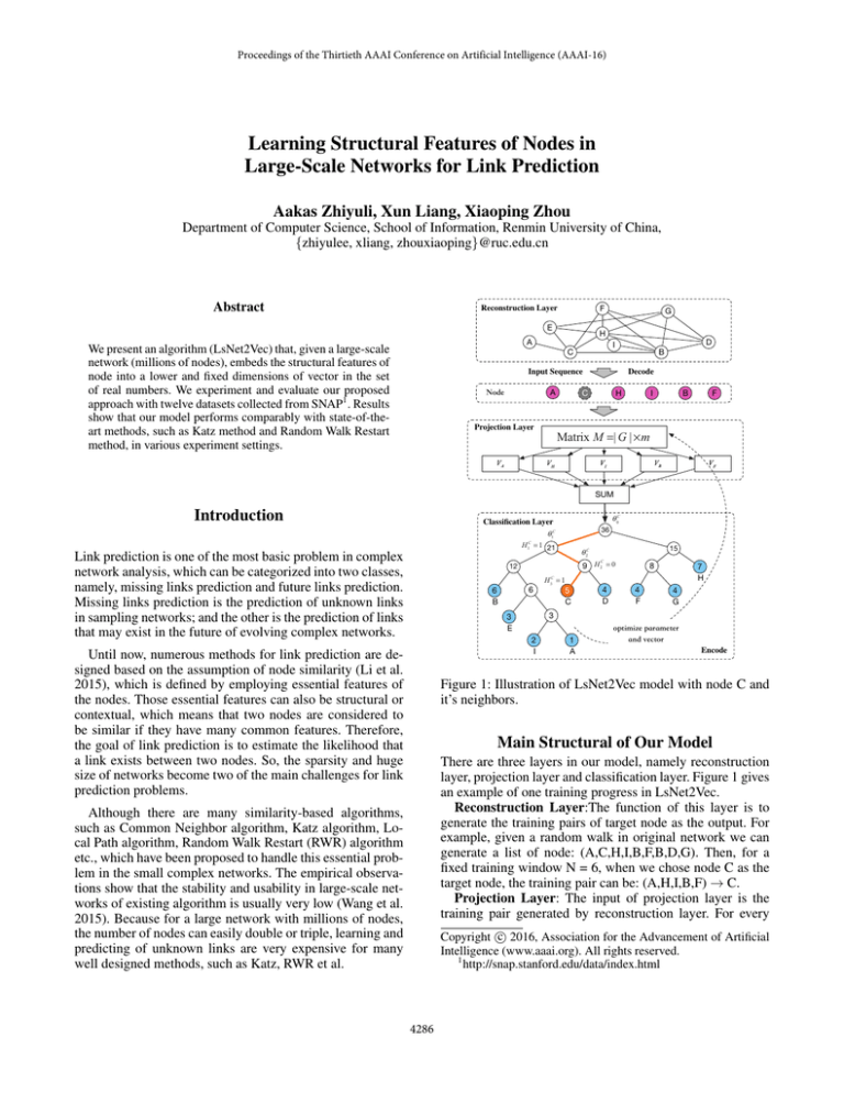
Figure 1: Illustration of LsNet2Vec model with node C and
it’s neighbors.
Main Structural of Our Model
There are three layers in our model, namely reconstruction
layer, projection layer and classification layer. Figure 1 gives
an example of one training progress in LsNet2Vec.
Reconstruction Layer:The function of this layer is to
generate the training pairs of target node as the output. For
example, given a random walk in original network we can
generate a list of node: (A,C,H,I,B,F,B,D,G). Then, for a
fixed training window N = 6, when we chose node C as the
target node, the training pair can be: (A,H,I,B,F) → C.
Projection Layer: The input of projection layer is the
training pair generated by reconstruction layer. For every
Although there are many similarity-based algorithms,
such as Common Neighbor algorithm, Katz algorithm, Local Path algorithm, Random Walk Restart (RWR) algorithm
etc., which have been proposed to handle this essential problem in the small complex networks. The empirical observations show that the stability and usability in large-scale networks of existing algorithm is usually very low (Wang et al.
2015). Because for a large network with millions of nodes,
the number of nodes can easily double or triple, learning and
predicting of unknown links are very expensive for many
well designed methods, such as Katz, RWR et al.
c 2016, Association for the Advancement of Artificial
Copyright Intelligence (www.aaai.org). All rights reserved.
1
http://snap.stanford.edu/data/index.html
4286
node in original network, we embed the node into a vector vi ∈ Rm . With a given training pair: N(C)=(A,H,I,B,F)
→ C, the projection layer computes the vector representations of target node’s neighbors in original network by taking a linear combination of the neighbor’s vectors: v(C) =
i∈N (C) vi .
Classification Layer: The input of classification layer is
the result from projection layer: (C, v(C) ). In classification
layer, we store all the nodes in the original network as a leaf
node in the Degree based Huffman tree (as shown in Figure 1, building based on the degree of nodes in original network). We denote the non-leaf nodes in the Huffman tree
as a classifier with logistic regression. So, the classification
layer for predicting the target node is based on its neighbors’ eigenvectors. Therefore, v(C) is using as an input of
root node in Huffman tree for classification, the object is to
make the probability of classification result becomes maximum according to the v(C) of leaf node C:
P C|
|
C
p vC v(C) =
p HjC v(C) , θj−1
Table 1: Results in red(∗) denote the best score while the
blue(♦) stands for the second best. The number under the
best score is the difference between the best and second best.
(1)
j=1
where, P C is the length of the path from root node to leaf
node C, HjC is the Huffman code of non-leaf node in the
path. So, for each i − th target node in training set, the cost
function of whole model is:
P i|
|
i
O = arg max
(2)
log
p Hji v(i) , θj−1
i∈V
0.01
0.0001
LP
RWR
0.935
0.974
0.972
0.975
0.922
0.969
0.955
0.958
0.897
0.904
0.957
0.954
0.956
D.set
L2V
CN
RA
ACN
0.990
0.933
CCN
0.988
0.921
EEN
0.979
∗1.5%
∗1.9%
∗2.2%
KA
♦
♦
♦
UEN
0.978
0.576
0.578
0.889
0.697
0.825
DCN
0.984
0.816
0.817
0.969
0.952
0.954
APN1
0.972
0.834
0.835
0.918
0.907
0.900
APN2
0.994
0.723
0.745
0.844
0.856
0.914
PRN
0.955
0.562
0.561
0.913
0.709
0.900
YSN
0.871
0.625
0.702
0.750
0.800
0.848
TRN
0.949
0.565
0.565
0.901
0.689
0.890
CRN
0.963
0.573
0.573
0.902
0.701
0.901
WTN
0.825
0.516
0.538
0.798
0.801
0.824
∗8.9%
∗1.5%
∗5.4%
∗8.0%
∗4.2%
∗2.3%
∗4.8%
∗6.1%
∗0.1%
♦
♦
♦
♦
♦
♦
♦
♦
♦
The results of AUC score show that our model performs comparably with state-of-the-art methods in largescale datasets. We argue that LsNet2Vec provides a fast
and best result in large-scale networks for the following
two main reasons: 1) the structural features of the node can
be better represented by the lower and fixed dimensions
vector that learned from the whole network with node cooccurrence. 2) the prediction method of LsNet2Vec can benefit from n-rank neighbors with a linear complexity increase
with n, and cosine measure can reduce the complexity of
the similarity measure in large-scale network between two
arbitrary nodes.
j=1
Finally, we use the stochastic gradient ascent (SGA)
method to optimize parameters and the vector representations in projection layer. When the training progress is over,
we can obtain the distributed representation of every node
with a fixed dimensions vector, and the similarity of node
pairs can be easily computed with the cosine measure in
large-scale networks.
Acknowledgments
The work was supported by the Fundamental Research
Funds for the Central Universities and the Research Funds
of Renmin University of China (10XNI029), the Beijing
NSF under grant number 4132067, the NSF of China under
grant numbers 71531012 and 71271211 and the program of
2015 Renmin University of China of training top talents with
spirit of innovation.
Experiment and Discussion
We conduct extensive experimental analyses on twelve famous datasets and present a controlled comparison of our
model against several strong baselines of link prediction
methods provided in Lu(2011). The baseline methods are
Common neighbor (CN), Resource Allocation (RA), Katz
(KA), Local Path (LP) and Random Walk Restart (RWR).
The node number of networks in table 1 range from
1.88 × 104 to 2.39 × 106 , and the edge number of networks
range from 1.83×105 to 5.02×106 . Experimental results are
reported as the area under the ROC curve (AUC). We divide
each network into training set and testing set randomly in every test. The number of the edges in training set is 9:1 with
testing set. Due to the huge amount of some networks, we
can’t calculate the similarity between every node as a whole
for some complex baseline methods, i.e. Katz, RWR. For a
fair comparison, we sample the community from the whole
network with depth-first and breadth-first separately for 100
times/network, and test the AUC score in every sample for
10 times.
References
Li, L.; Qian, L.; Cheng, J.; Ma, M.; and Chen, X. 2015.
Accurate similarity index based on the contributions of paths
and end nodes for link prediction. Journal of Information
Science 41(2):167–177.
Lü, L., and Zhou, T. 2011. Link prediction in complex
networks: A survey. Physica A: Statistical Mechanics and
its Applications 390(6):1150–1170.
Wang, X.; He, D.; Chen, D.; and Xu, J. 2015. ClusteringBased Collaborative Filtering for Link Prediction. 332–338.
Twenty-Ninth AAAI Conference on Artificial Intelligence.
4287