Proceedings of the Twenty-Ninth AAAI Conference on Artificial Intelligence
Machine Teaching:
An Inverse Problem to Machine Learning and
an Approach Toward Optimal Education
Xiaojin Zhu
Department of Computer Sciences, University of Wisconsin–Madison
Madison, WI, USA 53706
jerryzhu@cs.wisc.edu
Abstract
A
D
A(D)
I draw the reader’s attention to machine teaching, the problem of finding an optimal training set given a machine learning algorithm and a target model. In addition to generating
fascinating mathematical questions for computer scientists to
ponder, machine teaching holds the promise of enhancing education and personnel training. The Socratic dialogue style
aims to stimulate critical thinking.
∗
θ
−1 ∗
Α (θ )
−1
Α
Θ
D
D
Given a training set D 2 D, machine learning returns a
model A(D) 2 ⇥. Note A in general is many-to-one. Conversely, given a target model ✓⇤ 2 ⇥ the inverse function
A 1 returns the set of training sets that will result in ✓⇤ . Machine teaching aims to identify the optimal member among
A 1 (✓⇤ ). However, A 1 is often challenging to compute,
and may even be empty for some ✓⇤ . Machine teaching must
handle these issues.
Q: Isn’t machine teaching just active learning / experimental
design?
No. Recall active learning allows the learner to “ask
questions” by selecting items x and asking an oracle for its label y (Settles 2012). Consider learning a
noiseless threshold classifier in [0, 1], as shown below.
Of Machines
Q: I know machine learning; What is machine teaching?
Consider a “student” who is a machine learning algorithm, for example, a Support Vector Machine (SVM) or
kmeans clustering. Now consider a “teacher” who wants the
student to learn a target model ✓⇤ . For example, ✓⇤ can be
a specific hyperplane in SVM, or the location of the k centroids in kmeans. The teacher knows ✓⇤ and the student’s
learning algorithm, and teaches by giving the student training examples. Machine teaching aims to design the optimal
training set D.
Q: What do you mean by optimal?
One definition is the cardinality of D: the smaller |D| is,
the better. But there are other definitions as we shall see.
Q: If we already know the true model ✓⇤ , why bother training
a learner?
The applications are such that the teacher and the learner
are separate entities, and the teacher cannot directly “hard
wire” the learner. One application is education where the
learner is a human student. A more sinister “application”
is security where the learner is an adaptive spam filter, and
the “teacher” is a hacker who wishes to change the filtering
behavior by sending the spam filter specially designed messages. Regardless of the intention, machine teaching aims to
maximally influence the learner via optimal training data.
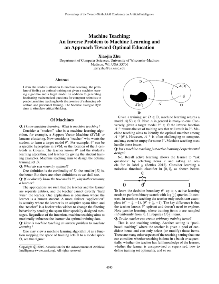
Q: How is machine teaching an inverse problem to machine
learning?
One may view a machine learning algorithm A as a function mapping the space of training sets D to a model space
⇥, see this figure:
ε
{
0
θ∗
1
To learn the decision boundary ✓⇤ up to ✏, active learning
needs to perform binary search with log( 1✏ ) queries. In contrast, in machine teaching the teacher only needs two examples: (✓⇤ 2✏ , 1), (✓⇤ + 2✏ , +1). The key difference is that
the teacher knows ✓⇤ upfront and doesn’t need to explore.
Note passive learning, where training items x are sampled
iid uniformly from [0, 1], requires O( 1✏ ) items.
Q: So the teacher can create arbitrary training items?
That is one teaching setting. Another setting is “poolbased teaching” where the teacher is given a pool of candidate items and can only select (or modify) those items.
There are many other aspects of the teaching setting that one
can consider: whether teaching is done in a batch or sequentially, whether the teacher has full knowledge of the learner,
whether the learner is unsupervised or supervised, how to
define training set optimality, and so on.
Copyright c 2015, Association for the Advancement of Artificial
Intelligence (www.aaai.org). All rights reserved.
4083
Q: The optimal teaching data D can be non-iid?
Yes, as the threshold classifier example shows. This is
most noticeable when optimality of D is measured by its
cardinality, but is in general true. It calls for new theoretical
analysis methods for machine teaching, whereas traditional
concentration inequalities based on iid-ness no longer apply.
Q: Did you just invent machine teaching?
No. What is new is our focus on tractable teaching computation for “modern” machine learners while generalizing the
definition of optimality beyond training set cardinality. But
there has been a long history of related work. The seminal
notion of teaching dimension concerns the cardinality of the
optimal teaching set (Goldman and Kearns 1995; Shinohara
and Miyano 1991). However, the learner’s algorithm A was
restricted to empirical risk minimization (specifically eliminating hypotheses inconsistent with training data). Subsequent theoretical developments can be found in e.g. (Zilles
et al. 2011; Balbach and Zeugmann 2009; Angluin 2004;
Angluin and Krikis 1997; Goldman and Mathias 1996;
Mathias 1997; Balbach and Zeugmann 2006; Balbach 2008;
Kobayashi and Shinohara 2009; Angluin and Krikis 2003;
Rivest and Yin 1995; Ben-David and Eiron 1998; Doliwa
et al. 2014). There are similar ideas in psychology, some of
them can be found in the references in (Patil et al. 2014).
Q: So you have a way to compute the optimal training set?
This is in general still an open problem, but we now understand the solution for certain machine teaching tasks (Zhu
2013; Patil et al. 2014). Specifically, we restrict ourselves
to batch teaching with full knowledge of the learning algorithm. The idea is as follows. Instead of directly computing
the difficult inverse function A 1 (✓⇤ ), we first convert it into
an optimization problem:
min
D2D
s.t.
✏(D)
(1)
A(D) = ✓⇤ .
(2)
Q: What is D under your minimization in (1)?
D is the search space of training sets. This is another design choice we must make. For example, we may decide
upfront that in D we want n/2 positive training examples
and n/2 negative ones, but the teacher can arbitrarily design each d dimensional feature vectors. The corresponding
search space can be
D = {{(xi , yi )1:n } | yi = ( 1)i , xi 2 Rd , i = 1 . . . n},
(6)
which is equivalent to Rnd . Such a continuous search space
is necessary for many standard optimization methods.
As another example, in pool-based machine teaching we
are given a candidate item set S. The training set D must be
a subset of S. Then D = 2S . Discrete optimization methods,
such as those based on submodularity, may be applicable
here (Krause and Golovin 2014; Iyer and Bilmes 2013; Bach
2013; Feige 1998; Krause and Guestrin 2005; Nemhauser,
Wolsey, and Fisher 1978).
Q: What about A(D) in (2)? Many machine learning algorithms do not have a closed-form solution w.r.t. the training
set D.
For some learners we are lucky to have a closed-form
A(D), and we can just plug in the closed-form expression. One example is ordinary least squares regression where
A(D) = (X > X) 1 X > y with D = (X, y). Another example is a Bayesian learner with a prior conjugate to D,
where A(D) is simply the posterior distribution (Zhu 2013;
Tenenbaum and Griffiths 2001; Rafferty and Griffiths 2010).
Yet another example is a kernel density estimator where
A(D) is written as a weighted sum of items in D (Patil et
al. 2014).
But you are right. For most learners, there is no closedform A(D). Nonetheless, a very large fraction of modern
machine learning algorithms are optimization-based. That
means the learner itself can be expressed as an optimization
problem of the form
This is not the final formulation – it will evolve later.
Q: OK. What is that ✏(D) objective?
✏(D) is a “teaching effort function” which we must define
to capture the notion of training set optimality. For example,
if we define
✏(D) = |D|
(3)
then we prefer small training sets. Alternatively, if we require the optimal training set to contain exactly n items we
may define
(4)
✏(D) = I|D|=n
where the indicator function Z = 0 if Z is true, and 1
otherwise. This teaching effort function is useful for designing human experiments as was done in (Patil et al.
2014). One can encode more complex notion of optimality with ✏(D). For example, in teaching a classification task
we may prefer that any two training items from different
classes be clearly distinguishable. Here, D is of the form
D = (x1 , y1 ), . . . , (xn , yn ). We may define
X
kxi xj k 1
(5)
✏(D) =
min
✓2⇥
s.t.
R(✓, D) + ⌦(✓)
(7)
g(✓)  0, h(✓) = 0.
(8)
Specifically, R(✓, D) is the empirical risk function, ⌦(✓) is
the regularizer, and g, h are constraints when applicable. For
these modern machine learners, we may replace A(D) in (2)
by the machine learning optimization problem. This turns
the original teaching problem (1) into a bilevel optimization
problem:
min
D2D
s.t.
✏(D)
✓⇤ 2 argmin✓2⇥ R(✓, D) + ⌦(✓)
s.t. g(✓)  0, h(✓) = 0.
(9)
(10)
(11)
In this bilevel optimization problem, the teaching objective (9) is known as the upper problem while the learning
problem (10) is the lower problem.
Q: Wait, I remember bilevel optimization is difficult.
True, and solving (9) in general is an challenge. For certain convex learners, one strategy is to further replace the
lower problem (10) by the corresponding Karush-KuhnTucker conditions. In doing so, the lower problem becomes
i,j:yi 6=yj
to avoid any near identical training items with different labels.
4084
a set of new constraints for the upper problem, and bilevel
optimization reduces to a single level optimization problem.
Q: I am still concerned. Constraints (2) and (10) looks
overly stringent; it is like matching a needle in a haystack.
I agree. The feasible sets can be exceedingly ill-formed.
One way to address the issue is to relax the teaching constraint such that the learner does not need to exactly learn
✓⇤ . Indeed, the original teaching problem (1) is equivalent to
min IA(D)=✓⇤ + ✏(D).
D2D
make predictions on some test items X and observe the predicted labels A(D0 )(X). The teacher can then eliminate all
A0 2 A where A0 (D0 )(X) 6= A(D0 )(X). This procedure
is repeated until A is sufficiently reduced. Then the teacher
finds the optimal training set for one of the remaining algorithms in A. An open question is how to make combined
probing and teaching optimal.
Q: You generalized the notion of teaching optimality from
|D| to arbitrary ✏(D). Is there a theory for ✏(D) similar to
teaching dimension?
This is another open question.
(12)
Recall the indicator function is Z = 0 if Z is true, and 1
otherwise. We may relax the indicator by another “teaching
risk function” ⇢() with a minimum at ✓⇤ :
min ⇢(A(D), ✓⇤ ) + ✏(D),
D2D
Of Humans
Q: What can machine teaching do for humans?
Machine teaching provides a unique approach to enhance
education and personnel training. In principle, we can use
machine teaching to design the optimal lesson for individual
students.
Q: There are already many intelligent computer tutoring
systems out there, and MOOC – what is unique about machine teaching?
Oversimplified, some existing education systems treat the
human learner as a black-box function f (D). The input D
is educational intervention, e.g. which course modules to offer to the student. The output of f (D) is the student’s test
score. The systems can make point evaluation of f at some
input D, and aim to maximize f based on such evaluations,
see e.g. (Lindsey et al. 2013). Being a black-box, the actual
learning process of the student is not directly modeled.
In contrast, machine teaching explicitly assumes a computational learning algorithm, or a cognitive model, A of
the student. Given educational intervention D, one may
first compute the resulting cognitive state A(D), which then
leads to the observed test score via an appropriate teaching
risk function ⇢(A(D), ✓⇤ ). Thus, machine teaching treats the
human learner as a “transparent box.” There is literature on
such cognitive models for tutoring (Koedinger et al. 2013).
Machine teaching’s focus is to explicitly compute the inverse A 1 to find the optimal lesson directly.
Q: What is the advantage of machine teaching?
The lesson will be optimal and personalized, given correct
cognitive model of the student.
Q: Isn’t “correct cognitive model” a strong assumption?
True. Like many things in mathematics, the more conditions one posits, the stronger the result. Of course, empirically the quality of the lesson will depend on the validity of
the cognitive model.
Q: Do we have the correct cognitive model for education?
Yes and no. For low level personnel training tasks such as
improving the performance of human categorization, there
are multiple well-established but competing cognitive models. On the other hand, accurate cognitive models for higher
level education is still a work in progress. The latter is currently the major limit on the applicability of machine teaching to education. However, the community does have useful
model fragments, and the machine teacher should take fully
advantage of them.
Q: So, is there indication that machine teaching works at all
on humans?
(13)
where is a weight that balances teaching risk and effort.
⇢() would measure the quality of the learned model A(D)
against the target model ✓⇤ . For example, a natural choice is
⇢(A(D), ✓⇤ ) = kA(D) ✓⇤ k, which measure how close the
learned model A(D) is to ✓⇤ in the parameter space with an
appropriate norm. As another example, for teaching a classifier we may measure the teaching risk by how much A(D)
and ✓⇤ disagree on future test data:
⇢(A(D), ✓⇤ ) = Ex⇠PX 1A(D)(x)6=✓⇤ (x)
(14)
where PX is the marginal test distribution; 1Z = 1 if Z is
true, and 0 otherwise; and we treat the models as classifiers.
We can then relax the bilevel optimization problem using
the teaching risk function ⇢() as follows:
min
D2D,⇠2⇥
s.t.
⇢(⇠, ✓⇤ ) + ✏(D)
(15)
(16)
⇠ 2 argmin✓2⇥ R(✓, D) + ⌦(✓)
s.t. g(✓)  0, h(✓) = 0. (17)
We can also bring the teaching effort function down as a
constraint ✏(D)  B within some budget B.
Q: There is still a glaring flaw: Can the teacher really have
full knowledge of the learning algorithm?
Good point. Under some circumstances this is plausible,
such as when the learner is a robot and the teacher has its
specifications. But when the learner is a human, we will rely
on established cognitive models in the psychology and education literature. We will turn our attention to human learners in the next part of the article.
Before that, though, I briefly mention a setting where the
teacher knows that the learning algorithm A is in a set A of
candidate learning algorithms, but not which one. As a concrete example, A may be the set of SVMs with different regularization weights. Note that, given the same training data
D, the learned model A(D) may be different for different
A 2 A. The teacher knows that the learner is an SVM but
doesn’t know its regularization weight.
A natural idea for this teaching setting is to “probe” the
learner. A simple probing strategy for classification is as follows. Start by teaching the learner with an initial training set
D0 . We assume the teacher cannot directly observe the resulting model A(D0 ). But the teacher can ask the learner to
4085
to a human student. Let D be the lesson, i.e., the training data, that the participant comes up with. Assuming human teacher is (near) optimal, we can then compare D to
A1 1 (✓⇤ ), . . . , Am1 (✓⇤ ) to identify the best matching cognitive model Aj . We may then view Aj as what the human
teacher assumes about the student. This is the strategy used
in (Khan, Zhu, and Mutlu 2011).
Yes. In (Patil et al. 2014) the authors studied a human
categorization task, where participants learn to classify line
segments as short vs. long. The assumed cognitive model
was a limited capacity retrieval model of human learners
similar to kernel density classifier. The teaching risk function ⇢() encodes the desire to minimize the expected future
test error.
Machine teaching identified an interesting optimal training set: the negative training items are tightly clumped together, so are the positive training items, and the negative
and positive items are symmetric but far away from the decision boundary, see figure below:
y=−1
0
Coda
Q: Now I am excited about machine teaching. What can I
do?
I call on the research community to study open problems
in machine teaching, including:
(Optimization) Despite our early successes in certain
teaching settings, solving for the optimal training data D is
still difficult in general. We expect that many tools developed in the optimization community can be brought to bear
on difficult problems like (15).
(Theory) Machine teaching originated from the theoretical study of teaching dimension. It is important to understand the theoretical properties of the optimal training set
under more general teaching settings. We speculate that information theory may be a suitable tool here: the teacher is
the encoder, the learner is the decoder, and the message is
the target model ✓⇤ . But there is a twist: the decoder is not
ideal. It is specified by whatever machine learning algorithm
it runs.
(Psychology) Cognitive psychology has been the first
place where machine teaching met humans. More studies
are needed to adjudicate existing cognitive models for human categorization. Human experiments also call for new
developments in machine teaching, such as the sequential
teaching setting (Bengio et al. 2009; Khan, Zhu, and Mutlu
2011; McCandliss et al. 2002; Kumar, Packer, and Koller
2010; Lee and Grauman 2011; Cakmak and Lopes 2012;
Pashler and Mozer 2013; Kobayashi and Shinohara 2009;
Balbach and Zeugmann 2009). More broadly, psychologists
have proposed cognitive models for many supervised and
unsupervised human learning tasks besides categorization.
These tasks form an ideal playground for machine teaching
practitioners.
(Education) Arguably more complex, education first
needs to identify computable cognitive models of the student. Existing intelligent tutoring systems are a good place
to start: with a little effort, one may hypothesize the inner
works of the student black-box. As a concrete example, at
University of Wisconsin–Madison we are developing a cognitive model for chemistry education.
(Novel applications) Consider computer security. As
mentioned earlier, machine teaching also describes the optimal attack strategy if a hacker wants to influence a learning
agent, see (Mei and Zhu 2015) and the references therein.
The question is, knowing the optimal attack strategy predicted by machine teaching, can we effectively defend the
learning agent? There may be other serendipitous applications of machine teaching besides education and computer
security. Perhaps you will discover the next one!
y=1
θ∗=0.5
1
This solution resembles the toy example earlier; the larger
separation between positive and negative items is due to a
wide kernel bandwidth parameter in the cognitive model that
fits noisy human behaviors.
Human participants indeed generalize better from this
training set computed by machine teaching, compared to
a control group who received iid uniformly sampled training sets. Both groups are tested on a test set consisting of a
dense grid over the feature space. The group who received
machine-teaching training set had an average test-set accuracy of 72.5%, while the control group 69.8%. The difference is statistically significant.
Q: That’s promising. Still, how do you know that you have
the correct cognitive model? I remember you said there are
other competing models.
As is often said – all models are wrong, some are more
useful. One may use the prior literature and data to come
up with the best hypothesized model. They may be good
enough for machine teaching to produce useful lessons.
While identifying such a model is an issue, it is also an opportunity – Strangely enough, another potential use of machine teaching in psychology is to adjudicate cognitive models.
Q: Really? How can machine teaching tell which cognitive
model is correct?
Different cognitive models correspond to different learning algorithms. Call these algorithms A1 , . . . , Am . Given a
teaching target ✓⇤ , machine teaching can compute the optimal training set A1 1 (✓⇤ ), . . . , Am1 (✓⇤ ) for each cognitive model, respectively. If previous result is any indication,
these optimal training sets will each be non-iid and idiosyncratic.
We can then conduct a human experiment where we teach
a participant using one of the m training sets, and test her on
a common test set. Comparing multiple participants’ test set
performance, we identify the best training set, say Aj 1 (✓⇤ ),
among A1 1 (✓⇤ ), . . . , Am1 (✓⇤ ). This could lend weight to
the j-th cognitive model Aj being the best cognitive model.
Q: Tell me more about it.
A variant is as follows. we conduct a different kind of
human experiment: we ask the participant to be a teacher,
and let the participant design a lesson intended to teach ✓⇤
4086
Acknowledgments
Kobayashi, H., and Shinohara, A. 2009. Complexity of
teaching by a restricted number of examples. In COLT.
Koedinger, K. R.; Brunskill, E.; de Baker, R. S. J.;
McLaughlin, E. A.; and Stamper, J. C. 2013. New potentials
for data-driven intelligent tutoring system development and
optimization. AI Magazine 34(3):27–41.
Krause, A., and Golovin, D. 2014. Submodular function maximization. In Tractability: Practical Approaches
to Hard Problems (to appear). Cambridge University Press.
Krause, A., and Guestrin, C. 2005. Near-optimal value of
information in graphical models. In UAI.
Kumar, M. P.; Packer, B.; and Koller, D. 2010. Self-paced
learning for latent variable models. In NIPS.
Lee, Y. J., and Grauman, K. 2011. Learning the easy things
first: Self-paced visual category discovery. In CVPR.
Lindsey, R.; Mozer, M.; Huggins, W. J.; and Pashler, H.
2013. Optimizing instructional policies. In NIPS.
Mathias, H. D. 1997. A model of interactive teaching. J.
Comput. Syst. Sci. 54(3):487–501.
McCandliss, B. D.; Fiez, J. A.; Protopapas, A.; Conway, M.;
and McClelland, J. L. 2002. Success and failure in teaching the [r]-[l] contrast to Japanese adults: Tests of a Hebbian
model of plasticity and stabilization in spoken language perception. Cognitive, Affective, & Behavioral Neuroscience
2(2):89–108.
Mei, S., and Zhu, X. 2015. Using machine teaching to
identify optimal training-set attacks on machine learners. In
AAAI.
Nemhauser, G. L.; Wolsey, L. A.; and Fisher, M. L. 1978.
An analysis of approximations for maximizing submodular
set functionsI. Mathematical Programming 14(1):265–294.
Pashler, H., and Mozer, M. C. 2013. When does fading
enhance perceptual category learning? Journal of Experimental Psychology: Learning, Memory, and Cognition.
Patil, K.; Zhu, X.; Kopec, L.; and Love, B. 2014. Optimal
teaching for limited-capacity human learners. In NIPS.
Rafferty, A. N., and Griffiths, T. L. 2010. Optimal language
learning: The importance of starting representative. 32nd
Annual Conference of the Cognitive Science Society.
Rivest, R. L., and Yin, Y. L. 1995. Being taught can be faster
than asking questions. In COLT, 144–151. ACM.
Settles, B. 2012. Active Learning. Synthesis Lectures on Artificial Intelligence and Machine Learning. Morgan & Claypool.
Shinohara, A., and Miyano, S. 1991. Teachability in computational learning. New Generation Computing 8(4):337–
348.
Tenenbaum, J. B., and Griffiths, T. L. 2001. The rational
basis of representativeness. 23rd Annual Conference of the
Cognitive Science Society.
Zhu, X. 2013. Machine teaching for Bayesian learners in
the exponential family. In NIPS.
Zilles, S.; Lange, S.; Holte, R.; and Zinkevich, M. 2011.
Models of cooperative teaching and learning. JMLR 12:349–
384.
I am grateful to many people with whom I had helpful discussions, including Michael Kearns, Robert Nowak,
Daniel Lowd, Timothy Rogers, Chuck Kalish, Bradley
Love, Michael Mozer, Joshua Tenenbaum, Tom Griffiths,
Stephen Wright, Michael Ferris, Bilge Mutlu, Martina Rau,
Kaustubh Patil, and Shike Mei. I also thank the anonymous
reviewers for their constructive comments. Support for this
research was provided in part by NSF grant IIS 0953219 and
by the University of Wisconsin–Madison Graduate School
with funding from the Wisconsin Alumni Research Foundation.
References
Angluin, D., and Krikis, M. 1997. Teachers, learners and
black boxes. In COLT, 285–297. ACM.
Angluin, D., and Krikis, M. 2003. Learning from different
teachers. Machine Learning 51(2):137–163.
Angluin, D. 2004. Queries revisited. Theoretical Computer
Science 313(2):175–194.
Bach, F. 2013. Learning with submodular functions: A convex optimization perspective. Foundations and Trends in
Machine Learning 6(2-3):145–373.
Balbach, F. J., and Zeugmann, T. 2006. Teaching randomized learners. In COLT, 229–243. Springer.
Balbach, F. J., and Zeugmann, T. 2009. Recent developments in algorithmic teaching. In The 3rd Intl. Conf. on
Language and Automata Theory and Applications, 1–18.
Balbach, F. J. 2008. Measuring teachability using variants of
the teaching dimension. Theor. Comput. Sci. 397(1-3):94–
113.
Ben-David, S., and Eiron, N. 1998. Self-directed learning
and its relation to the vc-dimension and to teacher-directed
learning. Machine Learning 33(1):87–104.
Bengio, Y.; Louradour, J.; Collobert, R.; and Weston, J.
2009. Curriculum learning. In ICML.
Cakmak, M., and Lopes, M. 2012. Algorithmic and human
teaching of sequential decision tasks. In AAAI.
Doliwa, T.; Fan, G.; Simon, H. U.; and Zilles, S. 2014.
Recursive teaching dimension, VC-dimension and sample
compression. JMLR 15:3107–3131.
Feige, U. 1998. A threshold of ln n for approximating set
cover. J. ACM 45(4):634–652.
Goldman, S., and Kearns, M. 1995. On the complexity
of teaching. Journal of Computer and Systems Sciences
50(1):20–31.
Goldman, S., and Mathias, H. 1996. Teaching a smarter
learner.
Journal of Computer and Systems Sciences
52(2):255–267.
Iyer, R. K., and Bilmes, J. A. 2013. Submodular optimization with submodular cover and submodular knapsack constraints. In NIPS.
Khan, F.; Zhu, X.; and Mutlu, B. 2011. How do humans
teach: On curriculum learning and teaching dimension. In
NIPS.
4087