Proceedings of the Twenty-Ninth AAAI Conference on Artificial Intelligence
Policy Tree: Adaptive Representation for Policy Gradient
Ujjwal Das Gupta
Erik Talvitie
Michael Bowling
Department of Computing Science
University of Alberta
ujjwal@ualberta.ca
Department of Computer Science
Franklin & Marshall College
erik.talvitie@fandm.edu
Department of Computing Science
University of Alberta
mbowling@ualberta.ca
Wall above?
Abstract
0.13 0.25
Much of the focus on finding good representations in
reinforcement learning has been on learning complex
non-linear predictors of value. Policy gradient algorithms, which directly represent the policy, often need
fewer parameters to learn good policies. However, they
typically employ a fixed parametric representation that
may not be sufficient for complex domains. This paper
introduces the Policy Tree algorithm, which can learn
an adaptive representation of policy in the form of a decision tree over different instantiations of a base policy.
Policy gradient is used both to optimize the parameters
and to grow the tree by choosing splits that enable the
maximum local increase in the expected return of the
policy. Experiments show that this algorithm can choose
genuinely helpful splits and significantly improve upon
the commonly used linear Gibbs softmax policy, which
we choose as our base policy.
1
0.5
1.0
No
Yes
0.07
Up
Right
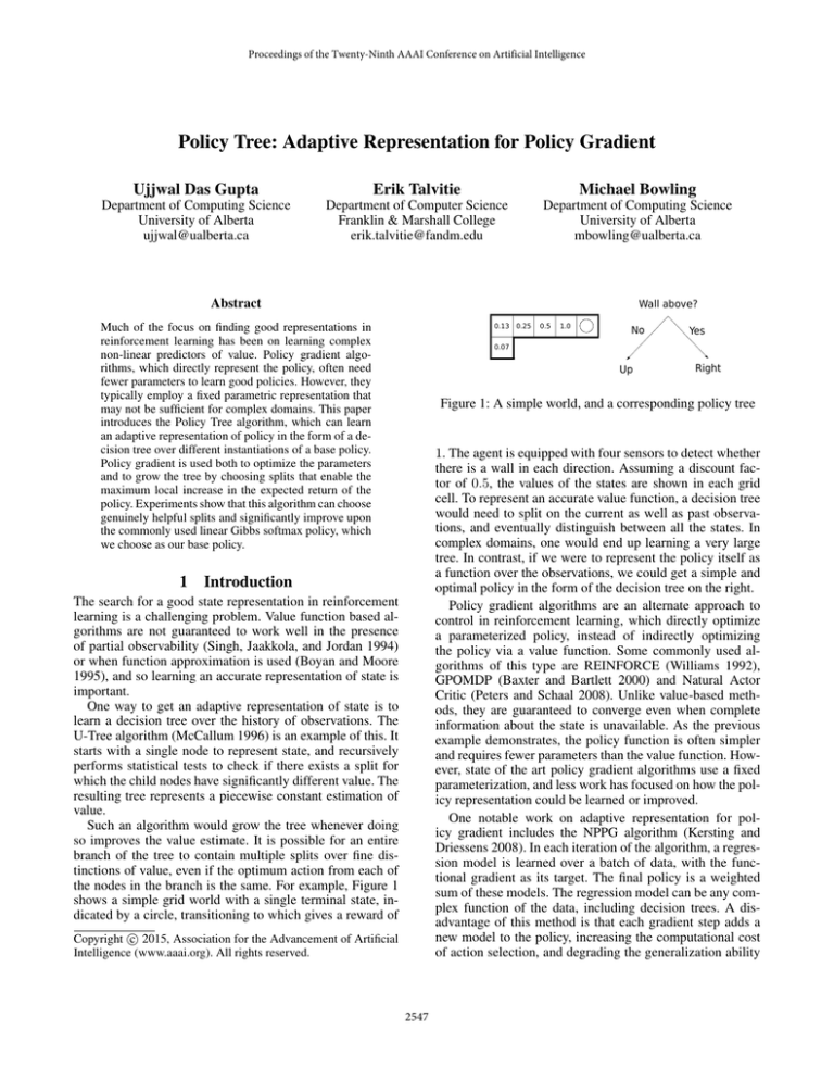
Figure 1: A simple world, and a corresponding policy tree
1. The agent is equipped with four sensors to detect whether
there is a wall in each direction. Assuming a discount factor of 0.5, the values of the states are shown in each grid
cell. To represent an accurate value function, a decision tree
would need to split on the current as well as past observations, and eventually distinguish between all the states. In
complex domains, one would end up learning a very large
tree. In contrast, if we were to represent the policy itself as
a function over the observations, we could get a simple and
optimal policy in the form of the decision tree on the right.
Policy gradient algorithms are an alternate approach to
control in reinforcement learning, which directly optimize
a parameterized policy, instead of indirectly optimizing
the policy via a value function. Some commonly used algorithms of this type are REINFORCE (Williams 1992),
GPOMDP (Baxter and Bartlett 2000) and Natural Actor
Critic (Peters and Schaal 2008). Unlike value-based methods, they are guaranteed to converge even when complete
information about the state is unavailable. As the previous
example demonstrates, the policy function is often simpler
and requires fewer parameters than the value function. However, state of the art policy gradient algorithms use a fixed
parameterization, and less work has focused on how the policy representation could be learned or improved.
One notable work on adaptive representation for policy gradient includes the NPPG algorithm (Kersting and
Driessens 2008). In each iteration of the algorithm, a regression model is learned over a batch of data, with the functional gradient as its target. The final policy is a weighted
sum of these models. The regression model can be any complex function of the data, including decision trees. A disadvantage of this method is that each gradient step adds a
new model to the policy, increasing the computational cost
of action selection, and degrading the generalization ability
Introduction
The search for a good state representation in reinforcement
learning is a challenging problem. Value function based algorithms are not guaranteed to work well in the presence
of partial observability (Singh, Jaakkola, and Jordan 1994)
or when function approximation is used (Boyan and Moore
1995), and so learning an accurate representation of state is
important.
One way to get an adaptive representation of state is to
learn a decision tree over the history of observations. The
U-Tree algorithm (McCallum 1996) is an example of this. It
starts with a single node to represent state, and recursively
performs statistical tests to check if there exists a split for
which the child nodes have significantly different value. The
resulting tree represents a piecewise constant estimation of
value.
Such an algorithm would grow the tree whenever doing
so improves the value estimate. It is possible for an entire
branch of the tree to contain multiple splits over fine distinctions of value, even if the optimum action from each of
the nodes in the branch is the same. For example, Figure 1
shows a simple grid world with a single terminal state, indicated by a circle, transitioning to which gives a reward of
c 2015, Association for the Advancement of Artificial
Copyright Intelligence (www.aaai.org). All rights reserved.
2547
(Da, Yu, and Zhou 2014). Additionally, the functional gradient, as the derivative of the value, could be as complex as
the value function itself. And so, as with value-based representation learning, a more complex representation may be
learned than is necessary.
In this paper, we describe a simpler approach to adaptive
representation for policy gradient, which we call the Policy
Tree algorithm. It aims to directly learn a function representing the policy, avoiding representation of value. This function takes the form of a decision tree, where the decision
nodes test single feature variables, and the leaves of the tree
contain a parameterized representation of policy. This kind
of representation has been studied in regression and classification scenarios (Gama 2004), but not in reinforcement
learning to our knowledge. The tree is grown only when doing so improves the expected return of the policy, and not
to increase the prediction accuracy of a value function or a
gradient estimate.
2
Figure 2: An example of the policy tree representation
When the actions belong to a continuous space, a common
parameterization of the policy is in the form of a Gaussian
distribution, with θµ and θσ being D-dimensional parameter vectors specifying the mean and standard deviation of
the distribution (Williams 1992):
πθ (a|φ) = N (a|µ(φ), σ(φ)),
where,
Reinforcement Learning & Policy Gradient
The reinforcement learning problem we consider involves an
agent which interacts with its environment at discrete time
steps t ∈ {1, 2, 3, ...}. At each time step, the agent perceives
its environment via a vector of features φ, selects an action
a ∈ A, and receives a scalar reward r ∈ R.
The agent chooses an action a at each time step by sampling a probability distribution πθ (a|φ), where θ represents
an internal parameterization of its policy. In episodic tasks,
the return of an episode is usually defined as the cumulative sum of rewards obtained. In continuing tasks, this sum
is unbounded, and the return is defined to be either the average reward per time step or a discounted sum of rewards.
The goal of a learning agent is to find the policy parameters which maximize the expected return from its interaction
with the environment, denoted as η(θ).
Policy gradient works by applying gradient ascent to find
a locally optimal solution to this problem. Note that computing the gradient ∇θ η(θ) would involve an expectation over
observed rewards, with the underlying probability distribution being a function of both the policy and the model of the
environment. The model is unknown to the agent, but a sample estimate of the gradient can be obtained by observing
trajectories of observations and rewards, while acting onpolicy. This is the principle underlying all policy gradient
algorithms, like REINFORCE, GPOMDP or Natural Actor
Critic. Some such algorithms additionally maintain a value
function estimate, which reduces the variance of the gradient
estimate (Sutton et al. 2000).
The actual policy can be any valid probability distribution
over actions that is differentiable with respect to all of its
parameters. That is, ∇θ πθ (a|φ) should exist. A commonly
used parametrization is the linear Gibbs softmax policy:
exp(θa T φ)
πθ (a|φ) = P|A|
,
T
i=1 exp(θi φ)
µ(φ) = θµ T φ,
σ(φ) = exp(θσ T φ),
1
(a − µ)2
N (a|µ, σ) = √
exp −
.
2σ 2
2πσ 2
3
(2)
The Policy Tree Algorithm
The Policy Tree algorithm represents its policy using a base
parametric policy and a binary decision tree. We assume that
the features are D-dimensional binary vectors φ ∈ {0, 1}D .
There exist methods, such as Coarse Coding, Tile Coding or
Kanerva Coding (Sutton and Barto 1998), which can convert
a space of real valued parameters into such a binary vector
space.
The internal nodes of the tree are decisions on an element
of the feature vector. We call the index of this element the
decision index of the node. Every feature vector φ maps to
one leaf node l(φ) in the tree, which is associated with a set
of parameters denoted by θl(φ) . The base policy at the leaf is
denoted by πθl(φ) (a|φ). This could be the linear Gibbs softmax policy (Equation 1), or the Gaussian policy (Equation
2), or any other differentiable policy function. If the linear
Gibbs softmax policy is chosen, θl(φ) contains D|A| parameters. A simple example of a policy tree is shown in Figure
2, in which, based on the feature vector φ, we use the base
policy instantiation corresponding to one of three leaf nodes
(L, L0 or L00 ) for action selection.
The high level procedure can be described as:
• Start with a single-node decision tree, with its root node
containing a randomly initialized parametrization of the
base policy. Repeat the following two stages alternatively:
– Parameter Optimization: Optimize all leaf node parameters using policy gradient for a fixed number of
episodes or time steps.
(1)
where θa is a D-dimensional vector of parameters corresponding to action a.
2548
– Tree Growth: Keep the parameters fixed for a number
of episodes or time steps, while the merit of each split
is judged. Choose a leaf node and a decision index on
which to split, according to our tree growth criterion.
Create two new children of this node, which inherit the
same policy parameters as their parent.
p=∞
p=1
During both of the stages, the action at each time step
is drawn from the policy function πθl(φ) (a|φ). We describe
in detail the two alternating stages of the algorithm in the
following sections.
3.1
Parameter Optimization
p=2
During this phase, the tree structure is kept fixed. Note that
∂
∂θ πθl(φ) (a|φ) is known to exist for θ ∈ θl(φ) , and is trivially 0 for θ ∈
/ θl(φ) , as πθl(φ) (a|φ) is not a function of
any such parameter. So, the policy function is differentiable
and the parameters can be optimized using any policy gradient technique. Convergence to a locally optimal solution is
guaranteed.
The per-step computational complexity during this phase
depends on the actual algorithm and parameterization used.
Most policy gradient algorithms have a complexity that is
linear in the number of parameters. In our case, the number
of parameters is NL NP , where NL is the number of leaf
nodes and NP is the number of parameters in the base policy
(NP = D|A| for the linear Gibbs softmax policy).
3.2
Figure 3: The p-norm spheres representing ||∆θ||p = the vectors θFL,k , θF 0 and θL0 for all L0 6= L. Note that
L,k
each ψL,k corresponds to a different policy function, which
we denote by πψL,k . Let η(ψL,k ) denote the corresponding
expected return.
Equation 3 ensures that πψl(φ),k (a|φ) = πθl(φ) (a|φ),
which means that all these policies have the same distribution over actions as the one represented by the existing
policy tree, even though the underlying representation has
changed. This ensures that we can measure the correct sample estimate of the gradient ∇ψL,k η(ψL,k ) by following the
policy of the tree. It is important to obtain a good estimate of
these gradients, to avoid splitting on noise. Therefore, during this phase, the policy is kept fixed while a suitably large
number of trajectories are observed, and ∇ψL,k η(ψL,k ) is
estimated for all L and k.
We choose the leaf node L and the decision index k to
split on using the following criterion:
Tree Growth
In this phase, the structure of the tree is altered by splitting
one of the leaf nodes, changing the underlying representation. In order to choose a good candidate split, we would
ideally like to know the global effect of a split after optimizing the resulting tree. This would require making every candidate split and performing parameter optimization
in each case, which is unrealistic and inefficient. However,
if we suggest a candidate split, and keep its parameters fixed,
the gradient of the expected return of this new policy function allows us to compute a first order approximation of the
expected return. This approximation is valid within a small
region of the parameter space, and can be used to measure
the local effect of the split. This is the basis of our criterion
to grow the tree. First, we describe a method to calculate the
gradients corresponding to every possible split in the tree.
A valid addition to the policy tree involves a split on one
of the leaf nodes, on a parameter k ∈ {1, ..., D}, such that k
is not a decision index on the path from the leaf node to the
root. For every leaf node L in the tree, and for every valid
index k, a pair of fringe child nodes are created, denoted as
0
FL,k and FL,k . They represent the child nodes of L which
would be active when φk = 1 and φk = 0, respectively.
Both of these nodes are associated with a parameter vector
which is the same as that of the parent leaf node, that is, for
all L and k:
θFL,k = θF 0 = θL .
(3)
L, k = arg max ||∇ψL,k η(ψL,k )||q .
(4)
L,k
It is worth reflecting on the interpretation of the q-norm of
the gradient vector, in order to interpret our criterion. By using a first order Taylor expansion of the expected return, we
can measure the change corresponding to a tiny step ∆ψ:
η(ψL,k + ∆ψ) = η(ψL,k ) + ∇ψL,k η(ψL,k )T ∆ψ. (5)
If we constrain ∆ψ to lie within a small p-norm sphere
with radius , we have:
max ∇ψL,k η(ψL,k )T ∆ψ = ||∇ψL,k η(ψL,k )||q ∆ψ
s.t. ||∆ψ||p ≤ (6)
1 1
where, + = 1.
p q
L,k
This shows that the q-norm of the gradient represents the
maximum change in the objective function within a local region of the parameter space bounded by the p-norm sphere,
where p and q are the dual norms of each other (Kolmogorov
Let ψL,k denote the combination of all the parameters
associated with the tree, when it is expanded to include the
0
pair of fringe nodes FL,k and FL,k . This is a combination of
2549
and Fomin 1957). Figure 3 shows a graphical representation
of various p-norm spheres.
By the same reasoning, ||∇θ η(θ)||q represents the maximum local improvement in the expected return that can be
obtained without altering the structure of the tree. A simple
stopping condition for tree growth is ||∇ψL,k η(ψL,k )||q <
λ||∇θ η(θ)||q , for some λ.
The fringe gradient ∇ψL,k η(ψL,k ) has (NL + 1)N P
components, as it is defined over all the parameters corresponding to an incremented tree. However, (NL − 1)N P
of these components are partial derivatives with respect to
the existing parameters in the tree, and are shared by all the
fringe gradients. Thus we need to measure at most NL D
gradients involving 2N P unique parameters, and the perstep computational complexity during this phase for most
policy gradient algorithms is O(NP NL D). For the linear
Gibbs softmax base policy, this is O(NL D2 |A|). Note that
the number of steps or episodes in this phase will almost
always be considerably lower than the previous one, as we
simply want a high accuracy gradient estimate and do not
need to optimize the parameters.
3.3
Fringe Bias Approximation
Figure 4: The graphical representation of the games. Clockwise from top-left, they are Monsters, Switcheroo, Mothership and Rescue
For many base policy functions, the number of parameters
will increase linearly with the number of features, making the complexity of the tree growth phase quadratic in
the number of features. Here, we describe an approximation which can reduce this complexity, and applies when the
base policy depends on linear functions of the features (as is
the case in Equations 1 and 2). If there are NF such functions, then the number of parameters NP is equal to NF D.
For example, with the linear Gibbs softmax policy we have
NF = |A|.
The standard practice when defining a linear function is to
augment the input vector φ with a bias term, usually chosen
as the first term of the vector. This term, denoted as φ0 , is always 1. If we had to choose a few components to represent
the gradient of the fringe parameters, choosing the parameters associated with φ0 is a reasonable approximation, which
0
we call the fringe bias approximation. Let ψL,k
denote the
subset of these parameters in ψL,k .
The bias parameters are always present regardless of the
observed features, and are thus indicative of the overall tendency of action selection. The other parameters are present
only when the corresponding features are active, and so they
can be thought of as context specific tendencies of action selection. The fringe bias approximation looks for features to
split on for which the policy would improve if different actions were preferred independent of the rest of the context.
However, it ignores improvements due to context specific
changes in action selection.
To apply the fringe bias approximation, we compute the
gradient of the expected return with respect to these bias pa0
rameters, or ∇ψL,k
η(ψL,k ). The tree growth criterion remains the same, which is to measure the norm of the gradient in this reduced space. By utilizing only the bias parameters, the computational complexity reduces by D and
becomes O(NL NF D) (or O(NL D|A|) for the linear Gibbs
softmax policy). As NP = NF D for such policies, the perstep complexity for tree growth becomes the same as that for
parameter optimization.
4
Experiments
We wish to evaluate the following questions empirically:
1. Can Policy Tree improve over the base policy?
2. How well does the fringe bias approximation perform?
3. Is the improvement merely due to an increase in the number of parameters, or does Policy Tree choose intelligent
splits?
To answer these questions, we consider a set of domains inspired by arcade games.
4.1
Domains
Our test suite is a set of 4 simple games inspired by arcade games, which have a 16x16 pixel game screen with
4 colours. A pictorial representation of them is presented in
Figure 4. All of these games are episodic with a maximum
episode length of 256 time steps, and every object moves
with a speed of one pixel per step. Objects in these games,
including the player agent, enemy agents, friendly agents or
bullets are a single pixel in size, and each object type is of a
distinct colour. Unless specified otherwise, the actions available to the agent are to move up, down, left, right or stay
still. The objective of the learning agent is to maximize the
expected undiscounted return.
For generating the binary feature vector, the location of
the player agent is assumed to be known. We divide the
2550
Rescue: The green player agent has to collect yellow
hostages and bring them to the blue rescue location to collect
a point. The rescue location is randomly located after every
successful rescue, and the player starts from a random location at the top of the screen. The hostages and red enemies
move across the screen horizontally at random intervals, and
collision with the enemies results in instant episode termination.
These games contain elements of partial observability and
non-linearity in the optimum policy function. As examples,
the direction of objects in the games cannot be determined
from a single game screen, and the best direction to move in
Monsters is conditional on multiple variables.
Figure 5: The feature mapping process.
game screen into zones, the size of which grows exponentially with the distance from the agent. Formally, if (x, y)
represents the displacement of a pixel from the agent, all
pixels with the same value of blog2 |x|c, blog2 |x|c, sgn(x)
and sgn(y) belong to the same zone. For each zone, we have
a feature corresponding to every colour used in the game. A
feature is set to 1 if an object of the corresponding colour
is found in that zone. An example of feature generation is
shown in Figure 5. The left image shows a game screen for
Mothership, with the black lines representing the zones centred around the agent. The right screen indicates the active
features in each zone via coloured dots (7 features are active
in this example). Such a choice of features allows fine distinctions to be made between objects near the agent, while
ensuring that the feature size grows only logarithmically
with the size of the game screen.
4.2
Experimental Setup
We use the linear Gibbs softmax policy as the base policy for
our algorithm, augmented with -greedy exploration. This
policy is defined as:
T
eθL,a φ
πθL (a|φ) = (1 − ) P|A|
.
+
Tφ
θ
|A|
L,i
i=1 e
(7)
The term ensures that the policy is sufficiently stochastic, even if θ takes on heavily deterministic values. This allows accurate estimation of the gradient at all times, and ensures that the policy does not quickly converge to a poor deterministic policy due to noise. Policy Tree benefits a great
deal from exploration, as often highly optimized parameters
are inherited from parent nodes, and need to be re-optimized
after a split. We noticed that adding this exploration term
helped the base policy as well.
We compare four different algorithms on these domains.
The first is the standard Policy Tree algorithm with the greedy Gibbs policy as the base. The second is a version
with the fringe bias approximation enabled. The third is a
version of the algorithm which chooses a random split during tree growth, for the purpose of testing whether the Policy
Tree is just benefiting from having a larger number parameters, or whether it makes good representation choices. And
finally, we test the base policy, which represents the standard
parametric approach to policy gradient.
We used the GPOMDP/Policy Gradient algorithm with
optimal baseline (Peters and Schaal 2006) to measure the
policy gradient in all of the algorithms. For Policy Tree,
we used a parameter optimization stage of 49000 episodes,
and a tree growth stage of 1000 episodes. Splits are therefore made after every 50000 episodes. The value of used
was 0.001. For the tree growth criterion, we choose the
q = 1 norm of the gradient. A stopping criterion parameter of λ = 1 was used.
For each algorithm, we performed 10 different runs of
learning over 500000 episodes. The average return was measured as the moving average of the total undiscounted return
per episode with a window length of 50000.
Monsters: The player agent is green. There are three red
monsters and three blue power suits randomly located in the
game area. The agent can collect and wear a power suit, allowing it to kill the next monster it collides with for one
point. A power suit lasts a maximum of 16 time steps once
it is worn. The monsters chase the agent when it is not powered, and stay still otherwise.
Switcheroo: There are two types of objects, red and blue.
At regular intervals, groups of 8 objects of a randomly chosen type move across the screen horizontally. The player
agent starts in the center of the screen, as an object of a random type. Hitting objects of the other type terminates the
episode, while hitting an object of the same type earns a
point. After a point is earned, the agent switches to the other
type.
Mothership: The blue mothership sits at the top of the
screen, while 4 rows of 8 red guard ships patrol horizontally
below. The green player agent is constrained to the bottom
of the screen, and cannot move up or down. It needs to shoot
the mothership to collect 5 points, and then shoot the guard
ships for 1 point each. Shooting the guards before destroying the mothership simply reflects bullets back at the agent,
and alerts the enemy, causing the mothership to move randomly, and the guard ships to shoot bullets. The agent is only
allowed to have one active bullet at a time, and there is a random wait of 0 or 1 time steps after its bullet is consumed. All
the bullets are coloured yellow.
4.3
Results
The learning curves of the Policy Tree algorithm as compared to the base policy are shown in Figures 6 to 9. The
2551
standard error in the results, across the 10 runs, is represented by the vertical error bars in the graphs. These results
allow us to answer the questions posed earlier. On our four
domains, we see that:
2.5
Average Return
2
1.5
1. The Policy Tree algorithm improves upon the underlying
base policy with statistical significance.
1
2. The fringe bias approximation trails the exact measure in
most domains, but improves over the linear parametrization significantly, without enduring additional computational complexity during tree growth.
Policy Tree
Policy Tree (Approx)
Random Splits
Base Policy
0.5
0
0
100000
200000 300000 400000
Number of Episodes
500000
3. An arbitrary increase in the number of parameters via
the random splitting does not improve performance at all.
This shows that the our tree growth criterion contributes
significantly to the effectiveness of the algorithm.
Figure 6: Results on Monsters
7
The Monsters domain shows the biggest improvement, as
well as the greatest gap between the exact and approximate
versions. In this domain, the feature that represents whether
or not the agent is powered is very informative. Policy Tree
chooses this as the first split in 80% of the runs, while this
drops to 20% with the approximation enabled. However, we
observed that the approximate version outperforms the base
policy even when this split is never made, indicating that the
chosen splits are not meaningless.
Average Return
6
5
4
3
2
Policy Tree
Policy Tree (Approx)
Random Splits
Base Policy
1
0
0
100000
200000
300000
Number of Episodes
400000
500000
5
There are a number of areas in which this work can be
expanded. The current version of our algorithm has fixed
lengths for the parameter optimization and tree growth
phases. One could test for convergence of the objective function during optimization, allowing the tree to get the best
possible performance before we try to expand the structure.
However, highly optimized policies tend to be highly deterministic, making re-optimization of the parameters after a
split trickier. The Gibbs policy, for instance, has a low gradient in regions of high determinism. It is possible that the use
of natural gradients would alleviate this problem, by measuring the change of the objective function with respect to
the actual change in the policy distribution, rather than the
change in parameter values.
The algorithm as described in this paper is restricted to
policy functions defined on binary features. However, in
general one could use any arbitrary base policy (defined, say,
on continuous features), as long as there exists a method to
perform a binary coding of these features, which the decision tree can split on. Future work could deal with better
ways to handle continuous features, similar to the Continuous U-Tree algorithm (Uther and Veloso 1998).
Due to the presence of noise in the gradients, or due to the
locality of our improvement measuring criterion, it is possible that some splits do not enhance the policy significantly.
This causes needless increase in the number of parameters,
and slows down learning by splitting the data available to
each branch. A possible fix for this would be to prune the
tree if optimization after a split does not significantly change
the parameters.
The splits in the decision tree are currently based on the
value of a single observation variable. In general, we could
Figure 7: Results on Switcheroo
20
18
Average Return
16
14
12
10
8
6
Policy Tree
Policy Tree (Approx)
Random Splits
Base Policy
4
2
0
0
100000
200000 300000
Number of Episodes
400000
500000
Figure 8: Results on Mothership
8
7
Average Return
6
5
4
3
2
Policy Tree
Policy Tree (Approx)
Random Splits
Base Policy
1
0
0
100000
200000
300000
Number of Episodes
400000
Future Work
500000
Figure 9: Results on Rescue
2552
Gama, J. 2004. Functional trees. Machine Learning
55(3):219–250.
Jie, T., and Abbeel, P. 2010. On a connection between
importance sampling and the likelihood ratio policy gradient. In Advances in Neural Information Processing Systems,
1000–1008.
Kersting, K., and Driessens, K. 2008. Non-parametric policy gradients: A unified treatment of propositional and relational domains. In Proceedings of the 25th International
Conference on Machine learning, 456–463. ACM.
Kolmogorov, A. N., and Fomin, S. V. 1957. Elements of the
theory of functions and functional analysis. Vol. 1, Metric
and normed spaces. Graylock Press.
McCallum, A. K. 1996. Learning to use selective attention
and short-term memory in sequential tasks. In From Animals to Animats 4: Proceedings of the Fourth International
Conference on Simulation of Adaptive Behavior, volume 4,
315. MIT Press.
Peters, J., and Schaal, S. 2006. Policy gradient methods for
robotics. In Intelligent Robots and Systems, 2006 IEEE/RSJ
International Conference on, 2219–2225. IEEE.
Peters, J., and Schaal, S. 2008. Natural actor-critic. Neurocomputing 71(7):1180–1190.
Singh, S. P.; Jaakkola, T.; and Jordan, M. I. 1994. Learning
without state-estimation in partially observable markovian
decision processes. In Proceedings of the 11th International
Conference on Machine Learning, 284–292.
Sutton, R. S., and Barto, A. G. 1998. Reinfocement Learning: An Introduction. MIT Press.
Sutton, R. S.; McAllester, D. A.; Singh, S. P.; and Mansour,
Y. 2000. Policy gradient methods for reinforcement learning with function approximation. In Advances in Neural Information Processing Systems 12 (NIPS 1999), 1057–1063.
MIT Press.
Uther, W. T., and Veloso, M. M. 1998. Tree based discretization for continuous state space reinforcement learning. In
Association for the Advancement of Artificial Intelligence,
769–774.
Williams, R. J. 1992. Simple statistical gradient-following
algorithms for connectionist reinforcement learning. Machine learning 8(3-4):229–256.
define a split over a conjunction or a disjunction of observation variables. This would increase the size of the fringe
used during tree growth, but would allow the algorithm to
find splits which may be significantly more meaningful. A
different kind of split in the decision nodes would be on a
linear combination of features. This can be viewed as a split
on a non-axis aligned hyperplane in the observation space.
As there are infinite such splits, it is not possible to measure
them using our fringe structure. However, there may be ways
to develop alternative criterion in order to grow a tree with
such a representation. Prior research suggests that such an
architecture is useful for classification but not for regression
(Breiman et al. 1984). It is unclear how useful it would be in
the search for an optimal policy.
The two phase structure of our algorithm is slightly sample inefficient, as the experience during tree growth is not
used to optimize the parameters. In our experiments, 2% of
the episodes are unused for optimization. Due to the requirement to stay on-policy to estimate the gradient, this is difficult to avoid. One possible solution would be to use importance sample weighting and utilize off-policy trajectories to compute the gradient. This would in fact avoid the
necessity of keeping the policy fixed during the tree growth
stage. The use of importance sampling in policy gradient has
been studied previously (Jie and Abbeel 2010). However,
the weights for the off-policy samples would reduce exponentially with the horizon of the problem, and we cannot
be certain whether it is possible to have a reliable off-policy
estimate of the gradient in most domains.
6
Conclusion
We presented the Policy Tree algorithm, and demonstrated
its utility on a variety of domains inspired by games. This
algorithm has the same convergence guarantees as parametric policy gradient methods, but can adapt its representation
whenever doing so improves the policy. We also present an
approximate form of this algorithm, which has a linear computational complexity per time-step in the number of parameters during the entire learning phase. We believe that these
results indicate that the gradient of the expected return is a
useful signal in the search for representation in reinforcement learning.
References
Baxter, J., and Bartlett, P. L. 2000. Direct gradient-based reinforcement learning. In Proceedings of the 2000 IEEE International Symposium on Circuits and Systems, volume 3,
271–274. IEEE.
Boyan, J., and Moore, A. W. 1995. Generalization in reinforcement learning: Safely approximating the value function. Advances in Neural Information Processing Systems
369–376.
Breiman, L.; Friedman, J.; Stone, C. J.; and Olshen, R. A.
1984. Classification and regression trees.
Da, Q.; Yu, Y.; and Zhou, Z.-H. 2014. Napping for functional representation of policy. In Proceedings of the International Conference on Autonomous Agents and MultiAgent Systems, 189–196.
2553