Proceedings of the Twenty-Ninth AAAI Conference on Artificial Intelligence
Building Effective Representations for Sketch Recognition
Jun Guo
Changhu Wang
Hongyang Chao
Sun Yat-sen University,
Guangzhou, P.R.China
Microsoft Research,
Beijing, P.R.China
Sun Yat-sen University,
Guangzhou, P.R.China
Abstract
As the popularity of touch-screen devices, understanding a user’s hand-drawn sketch has become an increasingly important research topic in artificial intelligence
and computer vision. However, different from natural
images, the hand-drawn sketches are often highly abstract, with sparse visual information and large intraclass variance, making the problem more challenging.
In this work, we study how to build effective representations for sketch recognition. First, to capture
saliency patterns of different scales and spatial arrangements, a Gabor-based low-level representation is proposed. Then, based on this representation, to discovery
more complex patterns in a sketch, a Hybrid Multilayer
Sparse Coding (HMSC) model is proposed to learn midlevel representations. An improved dictionary learning
algorithm is also leveraged in HMSC to reduce overfitting to common but trivial patterns. Extensive experiments show that the proposed representations are highly
discriminative and lead to large improvements over the
state of the arts.
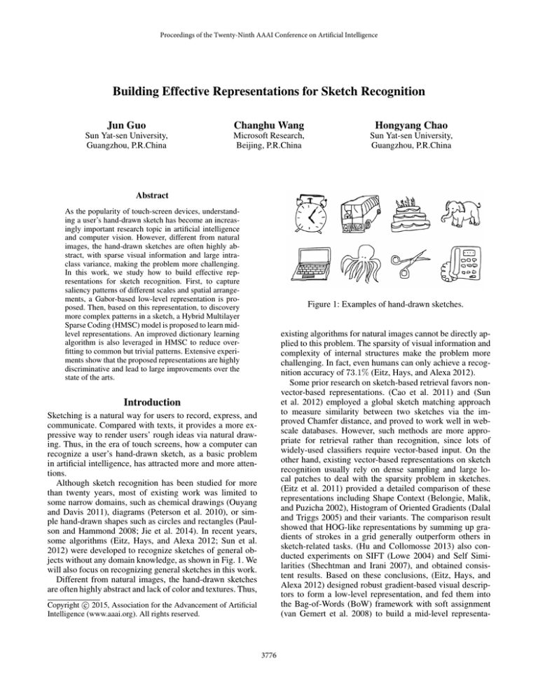
Figure 1: Examples of hand-drawn sketches.
existing algorithms for natural images cannot be directly applied to this problem. The sparsity of visual information and
complexity of internal structures make the problem more
challenging. In fact, even humans can only achieve a recognition accuracy of 73.1% (Eitz, Hays, and Alexa 2012).
Some prior research on sketch-based retrieval favors nonvector-based representations. (Cao et al. 2011) and (Sun
et al. 2012) employed a global sketch matching approach
to measure similarity between two sketches via the improved Chamfer distance, and proved to work well in webscale databases. However, such methods are more appropriate for retrieval rather than recognition, since lots of
widely-used classifiers require vector-based input. On the
other hand, existing vector-based representations on sketch
recognition usually rely on dense sampling and large local patches to deal with the sparsity problem in sketches.
(Eitz et al. 2011) provided a detailed comparison of these
representations including Shape Context (Belongie, Malik,
and Puzicha 2002), Histogram of Oriented Gradients (Dalal
and Triggs 2005) and their variants. The comparison result
showed that HOG-like representations by summing up gradients of strokes in a grid generally outperform others in
sketch-related tasks. (Hu and Collomosse 2013) also conducted experiments on SIFT (Lowe 2004) and Self Similarities (Shechtman and Irani 2007), and obtained consistent results. Based on these conclusions, (Eitz, Hays, and
Alexa 2012) designed robust gradient-based visual descriptors to form a low-level representation, and fed them into
the Bag-of-Words (BoW) framework with soft assignment
(van Gemert et al. 2008) to build a mid-level representa-
Introduction
Sketching is a natural way for users to record, express, and
communicate. Compared with texts, it provides a more expressive way to render users’ rough ideas via natural drawing. Thus, in the era of touch screens, how a computer can
recognize a user’s hand-drawn sketch, as a basic problem
in artificial intelligence, has attracted more and more attentions.
Although sketch recognition has been studied for more
than twenty years, most of existing work was limited to
some narrow domains, such as chemical drawings (Ouyang
and Davis 2011), diagrams (Peterson et al. 2010), or simple hand-drawn shapes such as circles and rectangles (Paulson and Hammond 2008; Jie et al. 2014). In recent years,
some algorithms (Eitz, Hays, and Alexa 2012; Sun et al.
2012) were developed to recognize sketches of general objects without any domain knowledge, as shown in Fig. 1. We
will also focus on recognizing general sketches in this work.
Different from natural images, the hand-drawn sketches
are often highly abstract and lack of color and textures. Thus,
c 2015, Association for the Advancement of Artificial
Copyright Intelligence (www.aaai.org). All rights reserved.
3776
Figure 2: Processing stages for building our local descriptors. For a clearer view, we don’t show the min-pooling step of the
pre-processing stage. That is, the initial input of the shown pipeline is a min-pooled sketch image.
avoid overfitting to trivial patterns with little discriminability. Based on the proposed representations, the recognition
accuracy on the benchmark dataset is improved to 68.5%
from the state-of-the-art 57.9%.
tion, which achieved the state-of-the-art performance. Jayasumana (Jayasumana et al. 2014) got slightly better results
by using an improved Kernel SVM classifier, keeping the
representations unchanged.
In spite of the success of Eitz’s representation (Eitz, Hays,
and Alexa 2012), there are still two main problems to restrict
its performance. First, its visual descriptors are built upon
fixed-size patches, with each patch uniformly divided into
square cells. Such neglect in scales and spatial arrangements
of local patterns cannot be compensated in higher-level representations, and thus limit the discriminability of the whole
model. The other disadvantage is from the over-simplified
mid-level representation. The BoW framework employed by
Eitz et al. used simple k-means algorithm to learn the midlevel representation, which is far from enough to further discover abstract and discriminative patterns.
Building Local Descriptors
The proposed low-level representation represents a sketch
by local descriptors. There are three processing stages to
build such a descriptor. The initial input is a local patch of
the sketch and the final output is a vector of N dimensions.
Before these three stages, a pre-processing stage for generating local patches is also involved. The whole pipeline is
shown in Fig. 2. We now describe each stage sequentially.
Pre-processing Stage
Each sketch image (zero pixel value for strokes and ones for
background) is rescaled via min pooling to guarantee that
the longer side is 224 pixels. Then, it is put in the center of
a blank image with an area of 256 × 256 to produce a blank
border with at least 16-pixel width. Such borders can reduce
the boundary effect that may occur during the execution of
some operations like filtering.
After that, sketch patches are extracted at points generated
by uniformly dense sampling on sketch images. To discover
patterns of different scales, multiple types of patches are extracted. In this work, we sample 32 × 32 points and utilize
square patches with sizes of 64 and 92 plus circular patches
with radii of 32 and 46.
To overcome these two problems, in this paper, we propose a novel model to represent hand-drawn sketches, including a Gabor-based low-level representation followed by
a sophisticated mid-level representation named Hybrid Multilayer Sparse Coding (HMSC). To solve the first problem,
in the low-level representation we first pre-processes the input sketch to reduce scale and translation variances. Then
patches of multiple sizes are extracted and Gabor transforms
are applied to decouple stroke orientations. Furthermore,
multiple pooling strategies are exploited to produce descriptors varying in scales and spatial arrangements, which are
further normalized and fed into HMSC. In order to fully
take use of these descriptors and discover more abstract
and discriminative sketch patterns, so as to solve the second problem, the HMSC representation is constructed with
sparse coding as the basic building block. First, in each Multilayer Sparse Coding (MSC) model, input features are processed through multiple layers of convolutional sparse coding, pooling and normalization sequentially. Then, multiple MSC models with different input descriptor types are
merged to result in the HMSC model, which encodes descriptors of various scales and spatial arrangements separately, and combines outputs from various layers. Moreover,
a mutual incoherence constraint is introduced to HMSC to
Stage 1: Transformation
The transformation stage maps a local patch to multiple
channels, each of which has the same resolution as the input
patch. More precisely, we apply real Gabor filters at each
patch pixels using R orientations and compute the magnitude response to generate R response channels. Note that
the wavelength of a real Gabor filter should not be too large
compared with its scale, so that the filter can provide narrow
orientation tuning. We have tried filters which give broader
orientation tuning, e.g., Eitz’s Gaussian’s first order derivative (Eitz, Hays, and Alexa 2012), but observed worse per-
3777
where is a small positive number.
Hybrid Multilayer Sparse Coding (HMSC)
(a) A 4 × 4 square grid
with bilinear weights
In this section we introduce the proposed mid-level representation, i.e., the Hybrid Multilayer Sparse Coding
(HMSC) model. First, the standard sparse coding algorithm
is briefly introduced, which is the building block of the
HMSC model. Then, an improved dictionary learning algorithm is presented to avoid overfitting to trivial sketch patterns. Finally, we discuss how to build the mid-level representation via the improved sparse coding algorithm in a
hybrid and multilayer manner.
(b) A 2 × 8 polar grid with bilinear weights
Figure 3: Two different pooling strategies used in our work.
Black spots in the image represent pooling centers.
Standard Sparse Coding
We need a more powerful model to encode the proposed local descriptors to a mid-level representation. Sparse coding
is adopted here as a building block of HMSC, since existing research has shown its encouraging performance compared with other encoding schemes like BoW (Boureau et
al. 2010). It tries to reconstruct all inputs using parsimonious
representations, the sparsity constraint of which makes it
possible to discover salient patterns that are hard to be manually explored and thus improve the discriminability. We first
briefly introduce the standard sparse coding in this section.
Let X be M local descriptors in an N -dimension vector space, i.e. X = [x1 , . . . , xM ] ∈ RN ×M . The key
idea of sparse coding is to represent vectors in X as linear
combinations of codewords taken from a learned dictionary
D = [d1 , . . . , dK ] ∈ RN ×K with sparse constraint. It can
be formulated as a matrix factorization problem with an L1norm penalty:
formance. This might because that sketch patches are composed of thin strokes, so that filters with narrow orientation tuning can better decouple multiple orientations at each
pixel, especially near the junctions of strokes.
In this work R is set to 9. The other parameters of Gabor
filters, i.e., the scale, the wavelength of the sinusoidal factor,
and the spatial aspect ratio are set to 5, 9, 1 respectively.
Stage 2: Pooling
Given R channels, the pooling stage spatially accumulates
pixel values in each channel, so that each channel is transformed into a vector of length C. All R resulting vectors are
concatenated to form a unnormalized descriptor of R × C
dimensions. Two pooling strategies are applied, hoping to
capture patterns of different spatial arrangements.
[Square Grid] We use a 4 × 4 square grid of pooling centers (Fig. 3(a)). Pixel values within a square channel are
summed spatially by bilinearly weighting them according to
their distances from the pooling centers. That is, the output
for each channel is a (C = 16)-dimension histogram consisting of 4 × 4 spatial bins.
min
D,Y
M
X
kxm − Dym k22 + λkym k1 ,
m=1
s.t. kdk k2 ≤ 1,
(2)
∀k = 1, 2, . . . , K,
where Y = [y1 , . . . , yM ] ∈ RK×M is a matrix containing
the associated sparse combinations (a.k.a. sparse codes), and
λ is the sparsity level.
The above optimization problem is convex for D (with
Y fixed) and Y (with D fixed) respectively, which can
be solved by alternatively optimizing D and Y (Lee et al.
2006).
[Polar Grid] A polar arrangement is adopted (Fig. 3(b)).
A circular channel is first divided into 2 distance intervals
and further uniformly split into 8 polar sectors. Then a histogram of (C = 8 × 2) dimensions is generated by summing up pixel values bilinearly weighted in polar coordinates. Besides, inspired by (Roman-Rangel et al. 2011), distance intervals are L2-normalized independently to balance
their contributions when building histograms.
Improved Dictionary Learning
Since sketch images are visually sparse and only consist of
several strokes, most local patches of sketches belong to
some simple but trivial patterns, e.g., a horizontal line, a
right angle, and so forth. Complex but discriminative patterns, such as a face which strongly suggests the existence
of a human-like sketched object, are infrequently observed.
Considering that the initial inputs of the sparse coding algorithm are descriptors extracted from local patches, the
learned dictionary might overfit to those frequent but unimportant patterns. To promote importance of less frequently
observed patterns so as to enrich codewords, we try to learn
a dictionary within which codewords are of highly mutual
incoherence. This idea is inspired by parts of works like
Stage 3: Normalization
The unnormalized descriptors from the previous stage are
combinations of histograms generated by summing up pixel
values, whose magnitudes vary over a wide range due to
the variations in stroke length. Thus, an effective normalization is needed to improve the performance. We experimented
with L1-norm and L2-norm normalizations, and found that
the latter was consistently better. Therefor, a descriptor x̄
from the previous stage is normalized by:
x̄
x= p
,
(1)
kx̄k22 + 3778
h × w adjacent vectors are concatenated in order to produce
(H − h + 1) × (W − w + 1) vectors of hwN dimensions.
These hwN -dimension vectors are then sparsely encoded,
while the dictionary is learned over sketches with a mutual
incoherence constraint (as discussed in the previous section).
(Tropp 2004), (Daubechies, Defrise, and De Mol 2004),
(Elad 2007) and (Eldar and Mishali 2009) which showed
that both the speed and accuracy of sparse coding depend on
the incoherence between codewords.
To achieve the above goal, we add a mutual incoherence
constraint in the standard sparse coding algorithm:
min
D,Y
M
X
[Stage 2: Pooling and Normalization] To further achieve
the property of translation-invariance and also reduce data
size, spatial max pooling is applied to aggregate sparse codes
from the previous stage.
For H ×W sparse codes generated by Stage 1 of all layers
except the final one, they are spatially divided into groups of
h × w vectors with an overlap ratio of 0.51j. Codes within
k
each group are max-pooled, resulting in H−h
+
1
×
h/2
j
k
W −w
w/2 + 1 pooled codes.
For sparse codes coming from Stage 1 of the final layer,
Spatial Pyramid Pooling (Lazebnik, Schmid, and Ponce
2006) is applied.
Pooled codes are then L2-norm normalized individually.
We have experimented with L1-norm normalization but did
not observe better results.
kxm − Dym k22 + λkym k1 ,
m=1
s.t. kdk k2 ≤ 1,
∀k = 1, 2, . . . , K,
kdTi dj k1 < η,
(3)
∀i, j = 1, 2, . . . , K, i 6= j,
where η is the mutual incoherence threshold. This optimization objective is somewhat similar to (Ramirez, Sprechmann, and Sapiro 2010), (Barchiesi and Plumbley 2013) and
(Bo, Ren, and Fox 2013), but the first one tried to promote
mutual incoherence of dictionaries rather than codewords
via an L2-norm penalty. The latter two ones focused on accuracy optimization algorithms. To accelerate the optimization process they required an L0-norm sparsity constraint to
strictly limit the number of nonzero elements, and thus are
not suitable here.
For efficiency, here we introduce an approximate algorithm to solve Eq. (3). We keep the learning phase and the
coding phase unchanged, but plug in a dictionary sweeping
phase between them.
More detailedly, in each iteration, after the learning phase
we sequentially scan each learned codeword. For a codeword di , if there exists another codeword dj (j > i) having
kdTi dj k1 ≥ η, i.e., violating the mutual incoherence constraint, di will be marked as obsolete. At the end of scanning, the swept dictionary may be composed of less than K
valid codewords and thus requires a supplement. In this case,
we simply go back to the input dataset X, sample some vectors from it, multiply their corresponding sparse codes and
the current dictionary so as to obtain their sparse approximations, and then compute the approximation errors. Sampled vectors with highest errors imply high independence of
the current codewords. Thus, we replace obsolete codewords
with these vectors. And the coding phase follows.
This simple algorithm proves to work very well according
to experiments.
Architecture of HMSC
A single MSC has the ability of learning mid-level representations in an unsupervised way. What’s more, by spatial pooling, the learned representations achieve the property of local translation invariance and are very stable. However, it only builds on one type of sketch patch, which limits
its power to discover patterns of different scales and spatial arrangements. Besides, although outputs produced by
the highest layers are robust and abstract, they miss some
local details which may be useful to distinguish highly similar sketch categories like armchair and chair. Therefore, the
proposed Hybrid Multilayer Sparse Coding (HMSC) model
further organizes multiple MSCs in a hybrid way, hoping to
exploit the advantages of MSC with its limitations reduced.
The whole pipeline of HMSC is shown in Fig. 4.
Generally speaking, HMSC encodes patches of various
scales and spatial arrangements, and combines outputs from
various layers. First, four types of patches, i.e., square
patches with an area of 642 and 922 , circular patches with
an area of 322 π and 462 π, are generated, from which descriptors are extracted. Descriptors from different types of
patches go through different one-layer MSCs and the outputs (named as S1.1, S1.2, C1.1 and C1.2 respectively) are
concatenated. To improve robustness to local deformations
and capture more abstract patterns, two-layer MSCs are also
exploited. Considering that the input for the second layer
has dropped lots of local details, to better render local structures, instead of building four two-layer MSCs individually,
pooled codes belonging to 64 × 64 and 92 × 92 square
patches are merged to be the input of the second layer. Similarly, pooled codes related to circular patches are concatenated and fed into the second layer. Outputs from these two
Multilayer Sparse Coding (MSC)
In this section we introduce the Multilayer Sparse Coding
(MSC) model, a simplified version of our HMSC. We will
introduce the architechture of HMSC in the next section.
MSC builds a representation layer by layer, with each
layer consisting of two stages. In the first layer, the input is
a set of local descriptors built upon one type of patch (e.g.,
square patches with an area of 642 ). In a higher layer, the
input is a set of pooled-and-normalized codes from its previous layer. We now describe each stage sequentially.
[Stage 1: Convolutional Sparse Coding] To consider the
spatial information and also to achieve local translation invariance, we perform convolutional coding. Given H × W
input vectors of N dimensions belonging to a sketch, every
1
For an easy explanation, we again use H, W, h and w to represent the number of input vectors and the number of adjacent vectors. We hope this slight overuse does not bring any ambiguity.
3779
Figure 4: Architecture of HMSC. Sketch patches of different types (including 64 × 64 / 92 × 92 square patches and 32 × 32 × π /
46×46×π circular patches) are generated from a min-pooled sketch and then encoded as local descriptors. These descriptors are
further fed into multiple layers of convolutional sparse coding (indicated as SC), with a pooling-and-normalization operation
(indicated as PN) inserted between SC layers. All sparse codes are finally transformed by a spatial-pyramid-pooling-andnormalization operation (indicated as SPN), and then concatenated to build the final representation, which is classified by a
linear SVM. For a clearer view, we only show 8 × 8 descriptors for the sketch.
two-layer MSCs (named as S2 and C2 individually) are also
combined with those from one-layer MSCs.
In our work, all one-layer MSCs learn dictionaries of
2000 codewords. For a two-layer MSC, the first layer learns
a 1000-codeword dictionary and its output is max-pooled
with the group size of 4 × 4, followed by the L2-norm normalization. Then comes the second layer which learns a dictionary of 2000 codewords. The final stage of each MSC applies a three-level Spatial Pyramid Max-Pooling with each
level generating 1 × 1, 2 × 2 and 3 × 3 pooled codes respectively. Note that although the final (concatenated) outputs are
indeed vectors of a high dimension, owning to the sparsity
they only require a small amount of memory and operating
them is usually efficient. We use the Liblinear package (Fan
et al. 2008) to learn a linear SVM for classification.
Hyper-parameters not mentioned, e.g. λ and η of sparse
coding, are automatically chosen via cross-validation.
Table 1: Mean classification accuracy and learning time of
different encoding schemes. Experiments were performed
on a laptop equipped with an Intel Core i7. BoW-Soft: Bagof-Words with soft assignment; SC-Std: standard sparse
coding; SC-Const: sparse coding with an L1-norm mutual
incoherence constraint, i.e., our approach.
Algorithm Mean Accuracy Learning Time
BoW-Soft
SC-Std
SC-Const
58.2%
61.7%
64.6%
18 min
30 min
32 min
Mutual Incoherence Constraint & Low-level
Representation
We investigated the effectiveness of the added mutual incoherence constraint on a one-layer MSC (including a 3 ×
3 convolutional sparse coding operation, a spatial pyramid max-pooling operation, and a normalization operation)
in terms of classification accuracy and learning time. We
learned a 2000-codeword dictionary on descriptors built
upon 64×64 square patches. To reduce experiment time, we
only sampled 1, 000, 000 descriptors for learning (no significant improvement was observed when using all descriptors).
As a baseline, we also encoded the proposed low-level representations using BoW with soft assignment (BoW-Soft) (van
Gemert et al. 2008). The results are shown in Table 1.
Experiments
In this section, we evaluate the proposed representations on
the largest sketch dataset collected by Eitz (Eitz, Hays, and
Alexa 2012), which contains 20, 000 sketches in 250 categories. This dataset is quite challenging as sketches in each
category are very diverse. Even humans can only achieve a
recognition rate of 73.1%. Following Eitz’s evaluation protocol, we partition the dataset into three parts and perform
three-fold cross-test: each time two parts are used for training and the remaining part for testing. The mean classification accuracy of three folds is reported.
[Dictionary Learning] We can see that, standard sparse
coding performed much better than Bag-of-Words (BoW)
with an acceptable time overhead, consistent with existing
3780
Figure 5: Classification accuracy of components of HMSC.
For the definition of S1.1, S1.2, S2, C1.1, C1.2 and C2,
please refer to previous sections and Fig. 4. Here we introduce several new symbols. S1: the combination of S1.1 and
S1.2; S1 + C1: the combination of S1 and C1; C1 and S2 +
C2 are defined similarly to S1 and S1 + C1 respectively; All:
S1 + C1 + S2 + C2.
Figure 6: Classification accuracy on the benchmark dataset.
SHC: shape context (Belongie, Malik, and Puzicha 2002);
HOOSC: histogram of orientation shape context (RomanRangel et al. 2011); HOG: histogram of oriented gradient (Dalal and Triggs 2005); Eitz: Eitz’s model (Eitz,
Hays, and Alexa 2012), Jay: Jayasumana’s improved model
(Jayasumana et al. 2014); Fisher: Fisher kernel (Perronnin,
Sánchez, and Mensink 2010); HSC: Hierarchical Sparse
Coding (Yu, Lin, and Lafferty 2011); M-HMP: Multipath
Hierarchical Matching Pursuit (Bo, Ren, and Fox 2013).
research. What’s more, it greatly outperformed Eitz’s model
(56.0%). Moreover, with the mutual incoherence constraint,
sparse coding achieved higher accuracy with comparable
learning time, verifying the effectiveness of learning a rich
dictionary with diverse codewords.
In short, the above three subsections have verified the usefulness of building representations at various scales, spatial
arrangements, and layers.
[Low-level Representation] Notice that here we adopted
a simplified version (single scale, single spatial arrangement) of our low-level representation. Nevertheless, directly
applying BoW on it has exceeded Eitz’s reported accuracy
(which also used BoW), indicating the effectiveness of our
low-level representation.
The rest experiments are based on the improved sparse
coding algorithm.
Compared with State of the Arts
To the best of our knowledge, the state of the arts in sketch
recognition on this benchmark dataset achieved the accuracies of 56.0% (Eitz, Hays, and Alexa 2012) and 57.9%
(Jayasumana et al. 2014). We also implemented some typical works in natural image recognition and shape analysis
(see Fig. 6), but did not observe better results.
As shown in Fig. 6, the performance of our proposed
model (68.5%) greatly outperformed the state of the arts.
It should be noted that, both Eitz’s and Jayasumana’s works
used a Kernel SVM for classification, while we applied a
linear one. By carefully selecting a more effective classifier,
our model has potential to reach a higher recognition rate. In
addition, recalling that humans can only reach an accuracy
of 73.1% on this dataset, our result is quite promising.
Mid-Level Representation
To verify the effectiveness of components of HMSC, we list
the recognition rate of each component in Fig. 5.
[Scale] By concatenating the outputs of S1.1 and S1.2, S1
performed better than both of them. Compared with C1.1 or
C1.2, C1 also brought large improvement. These two comparison results indicate that, by learning representations at
multiple scales, we can capture different nontrivial patterns,
resulting in performance improvement.
Conclusion
In this paper, we systematically studied how to build effective representations for sketch recognition. We designed
a Gabor-based low-level representation, based on which a
mid-level representation named Hybrid Multilayer Sparse
Coding was proposed. By learning sparse codes with an
additional constraint on various scales and spatial arrangements, and performing encoding through a varying number
of layers, the proposed representations achieved a promising
accuracy 68.5% (human’s accuracy being 73.1%), leading to
a large improvement over the state of arts 57.9%.
[Spatial Arrangement] Similarly, higher accuracy can be
obtained after merging the outputs of S1 and C1, or merging the outputs of S2 and C2. This shows that representations built on various spatial arrangements are complementary and can discover more discriminative patterns.
[Layer] Now we further investigate the effect of layers of
HMSC. As shown in Fig. 5, four one-layer MSCs (S1.1,
S1.2, C1.1, C1.2) performed surprisingly well, all of which
outperformed the state of the arts. Although the two-layer
MSCs (S2, C2) performed worse than one-layer ones, merging all MSCs (S1, S2, C1, C2) achieved the highest accuracy of 68.5%. This result confirms that outputs from different layers are good at modeling sketch structures at different
level of abstraction, and they can work together to make up
a better model.
Acknowledgments
This work was partially supported by NSF of China under
Grant 61173081 and Guangdong Natural Science Foundation, P.R.China, under Grant S2011020001215.
3781
References
Lazebnik, S.; Schmid, C.; and Ponce, J. 2006. Beyond
bags of features: Spatial pyramid matching for recognizing
natural scene categories. In Computer Vision and Pattern
Recognition, 2006 IEEE Computer Society Conference on,
volume 2, 2169–2178. IEEE.
Lee, H.; Battle, A.; Raina, R.; and Ng, A. Y. 2006. Efficient
sparse coding algorithms. In Advances in neural information
processing systems, 801–808.
Lowe, D. G. 2004. Distinctive image features from scaleinvariant keypoints. International journal of computer vision 60(2):91–110.
Ouyang, T. Y., and Davis, R. 2011. Chemink: a natural
real-time recognition system for chemical drawings. In Proceedings of the 16th international conference on Intelligent
user interfaces, 267–276. ACM.
Paulson, B., and Hammond, T. 2008. Paleosketch: accurate
primitive sketch recognition and beautification. In Proceedings of the 13th international conference on Intelligent user
interfaces, 1–10. ACM.
Perronnin, F.; Sánchez, J.; and Mensink, T. 2010. Improving the fisher kernel for large-scale image classification. In
Computer Vision–ECCV 2010. Springer. 143–156.
Peterson, E. J.; Stahovich, T. F.; Doi, E.; and Alvarado, C.
2010. Grouping strokes into shapes in hand-drawn diagrams. In AAAI, volume 10, 14.
Ramirez, I.; Sprechmann, P.; and Sapiro, G. 2010. Classification and clustering via dictionary learning with structured incoherence and shared features. In Computer Vision
and Pattern Recognition (CVPR), 2010 IEEE Conference
on, 3501–3508. IEEE.
Roman-Rangel, E.; Pallan, C.; Odobez, J.-M.; and GaticaPerez, D. 2011. Analyzing ancient maya glyph collections
with contextual shape descriptors. International Journal of
Computer Vision 94(1):101–117.
Shechtman, E., and Irani, M. 2007. Matching local selfsimilarities across images and videos. In Computer Vision
and Pattern Recognition, 2007. CVPR’07. IEEE Conference
on, 1–8. IEEE.
Sun, Z.; Wang, C.; Zhang, L.; and Zhang, L. 2012. Queryadaptive shape topic mining for hand-drawn sketch recognition. In Proceedings of the 20th ACM international conference on Multimedia, 519–528. ACM.
Tropp, J. A. 2004. Greed is good: Algorithmic results for
sparse approximation. Information Theory, IEEE Transactions on 50(10):2231–2242.
van Gemert, J. C.; Geusebroek, J.-M.; Veenman, C. J.; and
Smeulders, A. W. 2008. Kernel codebooks for scene categorization. In Computer Vision–ECCV 2008. Springer. 696–
709.
Yu, K.; Lin, Y.; and Lafferty, J. 2011. Learning image representations from the pixel level via hierarchical sparse coding. In Computer Vision and Pattern Recognition (CVPR),
2011 IEEE Conference on, 1713–1720. IEEE.
Barchiesi, D., and Plumbley, M. D. 2013. Learning incoherent dictionaries for sparse approximation using iterative
projections and rotations. Signal Processing, IEEE Transactions on 61(8):2055–2065.
Belongie, S.; Malik, J.; and Puzicha, J. 2002. Shape matching and object recognition using shape contexts. Pattern
Analysis and Machine Intelligence, IEEE Transactions on
24(4):509–522.
Bo, L.; Ren, X.; and Fox, D. 2013. Multipath sparse coding using hierarchical matching pursuit. In Computer Vision and Pattern Recognition (CVPR), 2013 IEEE Conference on, 660–667. IEEE.
Boureau, Y.-L.; Bach, F.; LeCun, Y.; and Ponce, J. 2010.
Learning mid-level features for recognition. In Computer
Vision and Pattern Recognition (CVPR), 2010 IEEE Conference on, 2559–2566. IEEE.
Cao, Y.; Wang, C.; Zhang, L.; and Zhang, L. 2011. Edgel
index for large-scale sketch-based image search. In Computer Vision and Pattern Recognition (CVPR), 2011 IEEE
Conference on, 761–768. IEEE.
Dalal, N., and Triggs, B. 2005. Histograms of oriented gradients for human detection. In Computer Vision and Pattern Recognition, 2005. CVPR 2005. IEEE Computer Society Conference on, volume 1, 886–893. IEEE.
Daubechies, I.; Defrise, M.; and De Mol, C. 2004. An iterative thresholding algorithm for linear inverse problems with
a sparsity constraint. Communications on pure and applied
mathematics 57(11):1413–1457.
Eitz, M.; Hildebrand, K.; Boubekeur, T.; and Alexa, M.
2011. Sketch-based image retrieval: Benchmark and bag-offeatures descriptors. Visualization and Computer Graphics,
IEEE Transactions on 17(11):1624–1636.
Eitz, M.; Hays, J.; and Alexa, M. 2012. How do humans
sketch objects? ACM Trans. Graph. 31(4):44.
Elad, M. 2007. Optimized projections for compressed sensing. Signal Processing, IEEE Transactions on 55(12):5695–
5702.
Eldar, Y. C., and Mishali, M. 2009. Robust recovery of
signals from a structured union of subspaces. Information
Theory, IEEE Transactions on 55(11):5302–5316.
Fan, R.-E.; Chang, K.-W.; Hsieh, C.-J.; Wang, X.-R.; and
Lin, C.-J. 2008. Liblinear: A library for large linear classification. The Journal of Machine Learning Research 9:1871–
1874.
Hu, R., and Collomosse, J. 2013. A performance evaluation of gradient field hog descriptor for sketch based image retrieval. Computer Vision and Image Understanding
117(7):790–806.
Jayasumana, S.; Hartley, R.; Salzmann, M.; Li, H.; and Harandi, M. 2014. Optimizing over radial kernels on compact
manifolds.
Jie, W.; Changhu, W.; Liqing, Z.; and Yong, R. 2014. Sketch
recognition with natural correction and editing. In AAAI.
3782