Proceedings of the Twenty-Eighth AAAI Conference on Artificial Intelligence
Sparse Learning for Stochastic Composite Optimization
Weizhong Zhang∗ , Lijun Zhang† , Yao Hu∗ , Rong Jin† , Deng Cai∗ , Xiaofei He∗
∗
State Key Lab of CAD&CG, College of Computer Science, Zhejiang University, Hangzhou, China
†
Dept. of Computer Science & Eng., Michigan State University, East Lansing, MI, U.S.A.
{zhangweizhongzju, huyao001, dengcai, xiaofeihe}@gmail.com, {zhanglij, rongjin}@cse.msu.edu
Abstract
vectors and trace norm for low rank matrixes. This problem is often referred to as sparse learning or sparse online
learning (Langford, Li, and Zhang 2009) which means only
one training example is processed at each iteration.
A popular approach toward SCO is stochastic composite
gradient mapping. The key idea is to introduce the regularizer Ψ(w) in the gradient mapping (Lin, Chen, and Pena
2011; Chen, Lin, and Pena 2012; Ghadimi and Lan 2012;
Xiao and others 2010). Given the current solution wt , it updates the solution by
In this paper, we focus on Stochastic Composite Optimization (SCO) for sparse learning that aims to learn
a sparse solution. Although many SCO algorithms have
been developed for sparse learning with an optimal convergence rate O(1/T ), they often fail to deliver sparse
solutions at the end either because of the limited sparsity
regularization during stochastic optimization or due to
the limitation in online-to-batch conversion. To improve
the sparsity of solutions obtained by SCO, we propose
a simple but effective stochastic optimization scheme
that adds a novel sparse online-to-batch conversion to
the traditional SCO algorithms. The theoretical analysis
shows that our scheme can find a solution with better
sparse patterns without affecting the convergence rate.
Experimental results on both synthetic and real-world
data sets show that the proposed methods are more effective in recovering the sparse solution and have comparable convergence rate as the state-of-the-art SCO algorithms for sparse learning.
wt+1 = arg min Lt (w) + ηt Ψ(w)
where Lt (w) = (w − wt )T ĝt + 12 kw − wt k22 . Here ĝt
is a stochastic gradient and is usually computed as ĝt =
∂f (w, zt ), where zt = (xt , yt ) is a randomly sampled training example. The main advantage of using stochastic composite gradient mapping for SCO is that the intermediate solutions obtained by (3) are likely to be sparse, due to the
presence of the sparse regularizer Ψ(w). Many variants of
composite gradient mapping have been proposed and studied for SCO (Chen, Lin, and Pena 2012; Ghadimi and Lan
2012; Lan 2012; Lin, Chen, and Pena 2011). In the case
when the loss function f (w, z) is strongly convex, one can
achieve the optimal convergence rate O(1/T ).
We should note that besides stochastic composite gradient mapping, any Stochastic Optimization (SO) methods can
also be used to solve SCO. Recent work (Hazan and Kale
2011; Rakhlin, Shamir, and Sridharan 2012) shows that with
a small modification on SGD, we can also achieve the convergence rate O(1/T ).
One problem with most SCO methods is that although the
intermediate solutions are sparse, the final solution may not
be exactly sparse because it is usually obtained by taking the
average of the intermediate solutions (Xiao and others 2010;
Ghadimi and Lan 2012), a procedure that is sometimes referred to as online-to-batch conversion (Littlestone 1989;
Dekel and Singer 2005). Several SCO approaches were proposed recently to address this limitation by only utilizing
the solution of the last iteration (Chen, Lin, and Pena 2012).
They are however short in enforcing the last solution to be
exactly sparse. This is because the magnitude of the sparse
regularizer Ψ(w) has to be reduced over iterations as the intermediate solutions approach the optimal one, and thus, can
Introduction
Many machine learning problems can be formulated into a
Stochastic Composite Optimization problem (SCO):
min
w∈W
φ(w) = F (w) + Ψ(w)
(1)
where F (w) = Ez=(x,y)∼PXY [f (w, z)], W is the convex
domain for the feasible solutions, f (w, z) is a loss function which is convex in W, Ψ(w) is a regularizer that controls the complexity of the learned classifier w, and PXY
is a joint distribution for the input pattern x and the output variable y. Since PXY is unknown, most optimization
methods approximate PXY by a finite number of samples
zi = (xi , yi ), i = 1, . . . , n, which are often called training
examples, leading to the following optimization problem:
n
min
w∈W
1X
b
φ(w)
=
f (w, zi ) + Ψ(w)
n i=1
(3)
w∈W
(2)
In this study, we will focus on the case when Ψ(w) is a
sparsity-inducing regularizer, such as `1 norm for sparse
Copyright c 2014, Association for the Advancement of Artificial
Intelligence (www.aaai.org). All rights reserved.
893
1.001
The main problem with most Sparse Online Learning is
that although the intermediate solutions are sparse, the final solution, after online-to-batch conversion, is likely to
be dense in the number of non-zeros entries. Finally, it is
worth pointing out that Sparse Online Learning is closely
related to the sparse recovery problem (Daubechies et al.
2010) that has been studied extensively. Many efficient algorithms (Daubechies et al. 2010; Chartrand and Yin 2008;
Becker, Bobin, and Candès 2011) have been developed for
sparse recovery that can achieve a linear convergence rate.
The only limitation of these algorithms is that they are designed for full gradients, instead of stochastic gradients, and
therefore are inapplicable to our case. We refer the audience
to (Daubechies et al. 2010) for a comprehensive treatment
of this subject.
35
ORDA
a−SGD
1
ORDA
a−SGD
34
0.999
33
L1−norm of w
ED of w
0.998
0.997
0.996
0.995
32
31
30
29
0.994
28
0.993
27
0.992
0.991
26
0
1
2
3
Iterations
4
5
0
1
4
x 10
2
3
Iterations
4
5
4
x 10
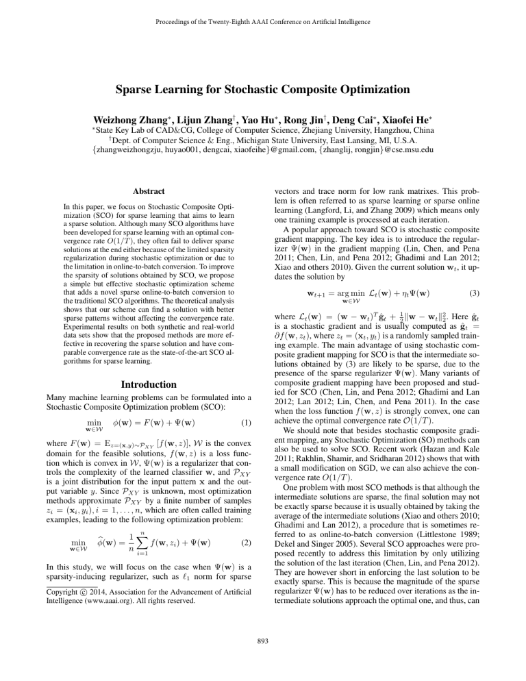
Figure 1: The exact sparsity (i.e. the percentage of non-zero
entries) (left) and `1 sparsity (right) of the solutions obtained
by α-SGD and ORDA over iterations
not force the final solution to be sparse, especially exactly
sparse.
To demonstrate our point, we conduct an experiment on
a synthetic dataset with λ = 1, ρ = 0.1, σe2 = 1(see the
experiment section for more details) using two sparse online
learning algoithms: α-SGD (Rakhlin, Shamir, and Sridharan
2012) that obtains the final solution by α-suffix averaging,
and ORDA (Ghadimi and Lan 2012) that takes the last solution as the final prediction model. Figure 1 (left) shows the
exact sparsity (i.e. the percentage of non-zero entries) over
iterations for the solutions obtained by these two algorithms.
It is clear that neither of these two approaches is able to obtain exactly sparse solutions, although the `1 sparsity of the
solutions is improved over iterations (Figure 1, right panel).
In this work, we develop a novel scheme for sparse learning that is likely to obtain exactly sparse solution. The proposed scheme is divided into two steps. In the first step,
we will run a standard SCO algorithm to obtain an approximately optimal solution w̄. In the second step, we introduce
a sparse online-to-batch conversion procedure that converts
e It is important to note
w̄ into an exactly sparse solution w.
that a simple rounding method may not work well for sparse
online-to-batch conversion. This is because through the iterations, the solution obtained by SCO is already subjected to
the rounding effect of Ψ(w) in the steps of composite gradient mapping. As a result, some of the small entries in the
final solution may be important for the prediction task, and
therefore simply removing small entries from the obtained
solution is unreliable as we will show in the empirical study
on real-world data (table 3).
Stochastic Optimization
Most Stochastic Optimization (SO) methods are based on
stochastic gradient descent (SGD). At each iteration, it obtains a stochastic gradient based on a randomly sampled
training example, and updates the solution by: wt+1 =
ΠW (wt − ηt ĝt ) , where ĝt is the stochastic subgradient of
φ(w), and Π is the projection operator of W. The original
SGD computes the final solution by taking the average of
the intermediate solutions, which achieves an O(log(T )/T )
convergence rate (Hazan et al. 2007) when the loss function
is strongly convex. This result is improved to O(1/T ) by
epoch gradient descent (Hazan and Kale 2011) and α-suffix
average (Rakhlin, Shamir, and Sridharan 2012). Although
both epoch gradient descent and α-suffix average achieve
the optimal convergence rate for strongly convex loss functions, they are not designed for sparse learning.
Stochastic Composite Optimization
The most popular methods for SCO are based on composite gradient mapping, which was firstly proposed for gradient descent in order to effectively explore the smoothness of
the objective function (Nesterov 2007). It was introduced to
online learning by (Xiao and others 2010) to obtain sparse
intermediate solutions. Multiple variants of composite gradient mapping were developed for Stochastic Optimization (Lin, Chen, and Pena 2011; Chen, Lin, and Pena 2012;
Ghadimi and Lan 2012; Xiao and others 2010). (Chen, Lin,
and Pena 2012) improves the convergence rate and sparsity
preserving ability of (Xiao and others 2010) by presenting a
novel algorithm of dual average, termed ORDA (stands for
optimal regularized dual average), that returns the last solution as the final prediction model. Although ORDA avoids
the problem of taking the average of intermediate solutions,
the learned prediction model is likely to be approximately
sparse, instead of exactly sparse, because the regularizer
used by the the last solution is usually too small (vanishes
rapidly over iterations).
Related Work
In this section, we only briefly review the recent work
on Sparse Online Learning, Stochastic Optimization and
Stochastic Composite Optimization.
Sparse Online Learning
Several algorithms have been developed for Sparse Online Learning (Duchi and Singer 2009; Langford, Li, and
Zhang 2009), where the goal is to generate a sequence of
sparse solutions that minimize the learner’s regret. Most of
the existed Sparse Online Learning algorithms are based
on composite gradient mapping or other rounding schemes
to remove the small entries in the intermediate solutions.
Preliminary and Notation
Similar to most Stochastic Optimization algorithms, we assume that we will randomly sample a training example
894
Algorithm 1 Sparse Learning based on Existing SCO Methods
1: Input: strong convexity λ ≥ 0, smoothness L ≥ 0,
tradeoff parameter 0 ≤ α ≤ 1, training examples {zt =
(xt , yt )}Tt=1 , and a Stochastic Composite Optimization
algorithm A.
2: Run A with the first (1 − α)T training examples
to obtain approximately optimal solution w̄1−α , i.e.,
w̄1−α = A(λ, L, (1 − α)T ).
3: // Sparse online-to-batch conversion:
4: Compute the average gradient at w̄1−α using the remaining αT training examples
z = (x, y) at each iteration, and obtain a stochastic gradient ĝ = ∂f (w, z) based on the sampled example. It is evie be the solution
dent that E[ĝ] = ∇Ez∼PXY [f (w, z)]. Let w
obtained after sampling T training examples. Our goal is to
e that on one hand minimizes the objective φ(w) and
find w
on the other hand is sufficiently sparse.
We denote w∗ ∈ W as the optimal solution that minimizes φ(w), i.e.
w∗ = arg min φ(w)
w∈W
Function f (w, z) is called λ-strongly convex if for any z and
all w, w0 ∈ W, we have
α
ḡ1−α
=
λ
f (w , z) ≥ f (w, z) + h∂f (w, z), w − wi + kw0 − wk22 .
2
0
0
Similarly, f (w, z) is L-smooth if for any z and all w, w0 ∈
W,
1
αT
T
X
∇f (w̄(1−α) , zi )
i=1+(1−α)T
e as
5: Compute the final solution w
α
e = argmin ḡ1−α
w
,w +
L 0
kw − wk22 .
2
Similar to most Stochastic Optimization algorithms, we
assume that f (w, z) is G-Lipschitz continuous, i.e.
k∂f (w, z)k ≤ G. Throughout this work, we assume that the
loss function f (w, z) is G-Lipschitz continuous, λ-strongly
convex, L-smooth and also kgt k ≤ G. Many loss functions
satisfy this condition, including regularized least square loss
and regularized logistic regression loss over bounded domains.
f (w0 , z) ≤ f (w, z) + h∂f (w, z), w0 − wi +
w∈W
L
2
kw − w̄1−α k + Ψ(w)
2
(4)
e
6: Return: w
in (4) without reducing its size, which will lead to an exe This is particularly clear when
actly sparse solution for w.
α
Ψ(w) = βkwk1 . If we note v = Lw̄1−α − ḡ1−α
, then the
solution to (4) can be given by
0,
if |[v]i | < β
e i=
[w]
1
[v
−
βsgn(v)]
,
else
i
L
The Proposed Stochastic Optimization Scheme
for Sparse Learning
We also note that the conversion step is different from a
simple rounding approach and the introduction of gradient
α
e
ḡ1−α
is important to ensure that the final sparse solution w
also minimizes the objective function φ(w). This is justified
by the following two theorems.
As described in the introduction section, the proposed
scheme is comprised of two steps. It learns an approximately optimal solution w̄ using a Stochastic Composite
Optimization (SCO) method at first, and then approximates
e through a novel onlinew̄ into an exactly sparse solution w
to-batch conversion procedure. Two specific approaches are
discussed in this section. In the first approach, any algorithm
for SCO with optimal convergence rate (e.g. α-suffix average (Rakhlin, Shamir, and Sridharan 2012)) can be used to
find an approximately optimal solution w̄, while in the second approach, the last solution obtained by a SGD is used
as w̄. For the convenience of presentation, we postpone the
detailed analysis to the appendix.
Theorem 1. Suppose the loss function f (w, z) is GLipschtiz continuous, λ-strongly convex and L-smooth. Assume SCO algorithm A is optimal that yields the following
generalization error bound
G2
E(φ(w̄1−α ) − φ(w∗ )) ≤ O
(1 − α)λT
Then, we have
Sparse Learning based on Existing SCO Methods
e − φ(w∗ )) ≤ O
E(φ(w)
Algorithm 1 shows the detailed steps of the first approach.
Firstly, it runs a SCO algorithm A with the first (1 − α)T
training examples, and computes an approximately sparse
solution w̄(1−α) . In the sparse online-to-batch conversion, it
calculates the gradient of w̄(1−α) using the remaining αT
training examples, and computes the final sparse solution
e by a composite gradient mapping in (4). Parameter α is
w
introduced to balance between Stochastic Composite Optimization and online-to-batch conversion. Unlike most SCO
methods where the size of sparse regularizer Ψ(w) is reduced over iterations, we use the original sparse regularizer
G2
G2
+
(1 − α)λT
αLT
As indicated by Theorem 1, the tradeoff parameter α balances the loss of Stochastic Composite Optimization and the
loss of sparse online-to-batch conversion: a small α will lead
to a small error in Stochastic Composite Optimization, but a
large error in the conversion step.
The theorem below refines Theorem 1 by presenting a
high probability bound.
Theorem 2. Let δ ∈ (0, 1/e) and assume T ≥ 4. Under
the same assumption as Theorem 1, with probability at least
895
1 − 2δ, we have
As indicated by Theorem 3, α is also a tradeoff parameter, which is the same with that of Algorithm 1. In addition,
the larger the α, the higher computational cost in online-tobatch conversion. So the parameter α allows us to balance
the tradeoff between computational cost and prediction accuracy. Finally, we observe that λ−2 in the bound of Theorem 3 is significantly worse than λ−1 in Theorem 1. This
may due to the loose bounds in our analysis, as the empirical study shows that Algorithms 1 and 2 give similar performance. We will examine in the future to see if a tighter
bound can be provided for Algorithm 2.
Theorem below refines the result in Theorem 3 with a high
probability bound.
Theorem 4. Let δ ∈ (0, 1/e), d is the length of vector gt
and assume T ≥ 4. Suppose the loss function f (w, z) is
G-Lipschtiz continuous, λ-strongly convex and L-smooth.
Then, with a probability at least 1 − 2δ, we have
L log(log(T )/δ)G2
e T ) − φ(w∗ ) ≤ O
φ(w
+
λ2 T
log((d + 1)/δ)G2
L log(log(T )/δ)G2
+
+
(1 − α)λ2 T
αLT
e − φ(w∗ )
φ(w)
G2 (log 2δ )2
log(log((1 − α)T )/δ)G2
≤O
+
λ(1 − α)T
αT
Sparse Learning Based on the Last Solution
One potential drawback of Algorithm 1 is that only a portion
of training examples will be used by the Stochastic Composite Optimization algorithm A to find approximately optimal
solution. To address this limitation, in the second approach,
we will use the last solution output from a standard stochastic gradient descent approach as the approximately optimal
solution, and apply an online-to-batch conversion procedure,
similar to Algorithm 1, to compute the final sparse solution
e Algorithm 2 gives the detailed steps. We observe that in
w.
contrast to Algorithm 1 that utilizes the first (1 − α)T training examples to learn w̄, all the training examples are used
to learn w̄, which may lead to a better usage of training examples. Similar to Algorithm 1, we introduce parameter α
that decides which portion of training examples will be used
for sparse online-to-batch conversion. Finally, since a similar conversion procedure is applied to convert w̄ to the final
e we expect w
e to be an exactly sparse solution
solution w,
benefited from the sufficiently large regularizer Ψ(w). The
e
theorems below show the optimality of w.
Experiments
In this section, we conduct experiments to evaluate the
performance of the proposed methods on two aspects: (i)
e is close to the optimal solution, and
whether the learned w
e will be sparse and recover most
(ii) whether the learned w
of the relevant features.
Three baseline algorithms will be used in our study.
• ORDA (Chen, Lin, and Pena 2012): an optimal Stochastic Composite Optimization algorithm that yields O(1/T )
convergence rate.
• α-SGD (Rakhlin, Shamir, and Sridharan 2012): an optimal algorithm for Stochastic Optimization.
• FOBOS (Duchi and Singer 2009): a Stochastic Composite
Optimization algorithm.
• OptimalSL: the proposed Algorithm 1 based on existing
SCO methods. And we take α-SGD as the algorithm A in
this experiment.
• LastSL: the proposed Algorithm 2 based on the last solution of SGD.
Algorithm 2 Sparse Learning based on the Last Solution
1: Input: strong convexity λ ≥ 0, smoothness L ≥ 0, ratio
0 ≤ α ≤ 1, and training examples {zt = (xt , yt )}Tt=1 ,
2: Initialize w1 = 0
3: for t = 1 to T do
4:
Compute the stochastic gradient ĝt = ∇f (w, zt )
5:
Update
wt+1 = ΠW (wt − ηt (ĝt + ∂Ψ(wt ))
where ηt = 1/(λt).
6: end for
7: // Sparse online-to-batch conversion:
8: Compute
e = argminhĝα , wi +
w
w∈W
L
kw − wT k2 + Ψ(w)
2
where
1
ĝ =
αT
α
T
X
Experiments on the Synthesized Dataset
Experimental model and parameter setting Following (Chen, Lin, and Pena 2012), we consider solving a sparse
linear regression problem: minw∈Rd f (w) + h(w) where
f (w) = 12 Ea,b ((hw, ai − b)2 ) + ρ2 kwk22 and h(w) =
λkwk1 . Every entry of the input vector a is generated from
the uniform distribution U (−1, 1) and the response is given
by b = ha, w∗ i + , where the noise ∼ N (0, σe2 ), and
[w∗ ]i = 1 for 1 ≤ i ≤ d2 and 0 otherwise. We set
λ = 0.1, ρ = 0.1, d = 100, and vary σe in the range
[1, 2, 3, ..., 10] in our experiments. The number N of training examples is set to be 50, 000. In addition, we set the
α = 0.1 for α-SGD and two proposed methods. It is easy to
∇f (wt , zt )
t=(1−α)T +1
e
9: Return: w
Theorem 3. Suppose the loss function f (w, z) is GLipschtiz continuous, λ-strongly convex and L-smooth.
Then, we have
2
G L
G2 L
G2
e − φ(w∗ )) ≤ O
E(φ(w)
+
+
λ2 T
(1 − α)λ2 T
αLT
896
line algorithms. From the running time, we can see that our
methods are more effective than FOBOS and ORDA. Figures 2 and 3 show the objective function’s values of different algorithms over iterations under different noise level σe .
We observe that the proposed algorithms are comparable to,
if not better than, the baselines in reducing the value of the
objective function.
Table 1: Numerical results on l1 regularized linear regression
problem with λ = 0.1, ρ = 0.1.
d = 100, N = 50000
σe2 = 1
Obj
ED
TD
SSR
RT
FOBOS
5.7099 0.99 0.99 0.671 0.5443
α-SGD
5.6984 1.00 1.00 0.667 0.3992
ORDA
5.7031 0.99 0.56 0.700 1.4690
LastSL
5.6968 0.50 0.50 1.000 0.4367
OptimalSL 5.6954 0.50 0.50 1.000 0.3772
d = 100, N = 50000
σe2 = 4
Obj
ED
TD
SSR
RT
FOBOS
7.2124 0.99 0.99 0.669 0.5172
α-SGD
7.2035 1.00 1.00 0.667 0.3901
ORDA
7.2096 0.99 0.65 0.669 1.4517
LastSL
7.2001 0.50 0.50 0.997 0.4281
OptimalSL 7.1976 0.50 0.50 1.000 0.3639
d = 100, N = 50000
σe2 = 25
Obj
ED
TD
SSR
RT
FOBOS
17.7351 1.00 1.00 0.667 0.5345
α-SGD
17.7437 1.00 1.00 0.667 0.3971
ORDA
17.7606 1.00 0.91 0.667 1.4546
LastSL
17.7339 0.62 0.62 0.897 0.4292
OptimalSL 17.7128 0.52 0.52 0.983 0.3746
d = 100, N = 50000
σe2 = 100
Obj
ED
TD
SSR
RT
FOBOS
55.3119 1.00 1.00 0.667 0.4252
α-SGD
55.406 1.00 1.00 0.667 0.3140
ORDA
55.4296 1.00 1.00 0.667 1.1707
LastSL
55.4195 0.82 0.82 0.757 0.3451
OptimalSL 55.3109 0.75 0.75 0.807 0.2971
8.5
ORDA
a−SGD
FOBOS
OptimalSL
LastSL
8
Objectives
7.5
7
6.5
6
5.5
0
1
2
3
4
Iterations
5
4
x 10
Figure 2: Objective values with parameter ρ = 0.1, λ =
0.1, σe2 = 1
70
ORDA
a−SGD
FOBOS
OptimalSL
LastSL
65
Objective
verify that under the above assumptions for a and b, we have
1
1
1 2
T
2
∗ 2
2 Ea,b ((a w − b) ) = 6 kw − w k2 + 2 σe , so we can calculate the exact objective function value and the optimal so7
lution fortunately: [w∗ ]i = 13
for i ≤ 50 and 0, otherwise.
Evaluation metrics To evaluate the properties of the
e we follow (Lin, Chen, and Pena 2011), and
learned w,
e
measure the objective function value and the sparsity of w
over iterations. Two metrics are used to measure the sparsity of a solution: the exact density ratio (ED for short),
Pd
that is computed as d1 i=1 I([w]i 6= 0), and the truncated sparse ratio (TD for short), which is computed as
Pd
1
−6
in our
i=1 I(|[w]i | > r ), where r is set to be 10
d
experiment. We also measure the recovery of the support set
of w∗ by SSR(w) = 2|S(w)∩S(w∗ )|/(|S(w)|+|S(w∗ )|),
where S(w) is the support set of w, which is composed of
the nonzero components of w, |S(w)| means the cardinality
of the set S(w). In addition, we give the running time (RT
for short, second). We run each experiment 100 times, and
report the results averaged over 100 trials.
Experimental results Table 1 summarizes the evaluation
results for the final solutions output from different algorithms under different noise level σe . We observe that besides yielding comparable value for the objective function,
the solutions found by the two proposed algorithms are significantly sparser than the ones found by the other base-
60
55
0
1
2
3
Iterations
4
5
4
x 10
Figure 3: Objective values with parameter ρ = 0.1, λ =
0.1, σe2 = 100
Experiments on Real-world Dataset
Dataset To further demonstrate the effectiveness of our
methods, we conduct an experiment on the well-known
MNIST dataset because it is easy to visualize the learned
prediction model. It is composed of the images for 10 digits
(0-9). Each image is a 28 × 28 gray-scale pixel map, which
can be treated as a real-valued vector of 784 dimension. Each
digit has roughly 6, 000 training examples and 1, 000 testing
examples.
Experimental model and parameter setting Following
the experiment setting in (Xiao and others 2010), we ap-
897
Experimental results According to table 2, we observe that
the proposed methods significantly improve the sparsity of
solutions compared to the baseline methods, and at the same
time, achieve comparable test errors. This is further confirmed by the grey-level images shown in Figure 4, in which
the solutions obtained by the proposed algorithms have significantly larger black areas than the other algorithms in
comparison.
Table 2: numerical results when we classify the digits 2 and
3
λ, ρ
Algorithms Test Error
ED
TD
FOBOS
0.0499
0.394 0.394
ρ = 0.01
α-SGD
0.0475
0.825 0.822
ORDA
0.0513
0.404 0.352
λ = 0.02
LastSL
0.0488
0.276 0.276
OptimalSL
0.0476
0.269 0.269
FOBOS
0.0578
0.375 0.375
ρ = 0.01
α-SGD
0.0529
0.825 0.822
ORDA
0.0573
0.382 0.329
λ = 0.03
LastSL
0.0558
0.223 0.223
OptimalSL
0.0528
0.199 0.199
FOBOS
0.0630
0.346 0.346
ρ = 0.01
α-SGD
0.0578
0.825 0.823
ORDA
0.0593
0.356 0.304
λ = 0.04
LastSL
0.0600
0.174 0.174
OptimalSL
0.0577
0.153 0.153
FOBOS
0.0672
0.334 0.334
ρ = 0.01
α-SGD
0.0617
0.825 0.823
ORDA
0.0651
0.341 0.294
λ = 0.05
LastSL
0.0638
0.144 0.144
OptimalSL
0.0610
0.125 0.125
Figure 4: The visualization for the prediction models learned
to classify between digits 2 and 3. Columns (a)-(d) are the
results for ρ = 0.01 and λ = 0.02, 0.03, 0.04, 0.05.
ply the regularized logistic regression to learn a binary classification model for each of the 45 pairs of digits. We set
e z) = log(1 + exp(−y(wT x +
the loss function as f (w,
ρ
2
e 2 , where w ∈ R784 , b is the model bias and
b))) + 2 kwk
e
e z)
w = [w; b]. It is straightforward to verify that f (w,
is a strongly convex and smooth loss function. We set the
sparsity-inducing regularizer Ψ(w) = λkwk1 . In our experiment, we fix ρ = 0.01, and vary λ from 0.02 to 0.05.
Parameter α is set to be 0.1 for α-SGD and the proposed
algorithms.
Evaluation metrics We evaluate the learned prediction
model by test error, exactly sparse ratio (ED) and truncated
sparse ratio (TD), the threshold here is also 10−6 . We run
each algorithm 100 times, each with an independent random
shuffle of training examples. Because of the space limitation, we only report the results for classifying digits 2 and 3
in Table 2. The results of some other digit pairs can be found
in the supplementary document.
To visualize the sparse patterns of the learned prediction
e 0 for a learned solution
models, we first create a new vector w
e as follows
w
(
e i<0
0.5 [w]
0
e i>0
1 [w]
e ]i =
[w
(5)
e i=0
0 [w]
Table 3: the test error of ORDA after(Test Error1) and before(Test Error2) simple rounding
λ, ρ
Test Error1 Test Error2
ρ = 0.01, λ = 0.02
0.0513
0.0499
ρ = 0.01, λ = 0.03
0.0573
0.0578
ρ = 0.01, λ = 0.04
0.0593
0.0630
ρ = 0.01, λ = 0.05
0.0651
0.0672
Table 3 shows the results after and before the simple
rounding process when we classify the digits 2 and 3. The
threshold here is 10−6 . We can observe that the simple
rounding process sometimes will make the test error increase significantly. So this approach is unreliable, which
demonstrates our analysis in the introduction section.
Conclusions
In this paper, we propose a novel scheme for sparse learning that aims to learn an exactly sparse solution based on
Stochastic Composite Optimization. The key idea is to introduce a sparse online-to-batch conversion procedure that
approximates the solution learned by a SCO algorithm into
an exactly sparse solution. Two specific algorithms are developed, one based on the solution output from an existing
e 0 to a matrix of size 28 × 28 and visualWe then reshape w
ize it as a grey-level image. Evidently, the larger the black
area in the grey-level image, the sparser the solution is. Figure 4 shows the images for the prediction models learned by
different algorithms for classifying between digits 2 and 3.
898
Lin, Q.; Chen, X.; and Pena, J. 2011. A sparsity preserving stochastic gradient method for composite optimization.
Manuscript, Carnegie Mellon University, PA 15213.
Littlestone, N. 1989. From on-line to batch learning. In Proceedings of the Second Annual Workshop on Computational
Learning Theory, 269–284.
Nesterov, Y. 2007. Gradient methods for minimizing composite objective function. Core discussion papers.
Rakhlin, A.; Shamir, O.; and Sridharan, K. 2012. Making gradient descent optimal for strongly convex stochastic
optimization. In Proceedings of the 29th International Conference on Machine Learning, 449–456.
Xiao, L., et al. 2010. Dual averaging methods for regularized stochastic learning and online optimization. Journal of
Machine Learning Research 11(2543-2596):4.
SCO algorithm, and one based on the last solution of the
a simple SGD algorithm. We verify, both theoretically and
empirically, that the proposed algorithms will yield solution
that is exactly sparse and achieves an optimal convergence
rate. In the future, we plan to investigate sparse online-tobatch conversion for loss functions that are only strongly
convex but not necessarily smooth.
Acknowledgments
This work was supported in part by National Basic Research Program of China (973 Program) under
Grant 2011CB302206, National Natural Science Foundation of China under Grants (61125203, 61233011,
61222207, 91120302), National Program for Special Support of Top-Notch Young Professionals, National Science
Foundation (IIS-1251031) and Office of Naval Research
(N000141210431).
References
Becker, S.; Bobin, J.; and Candès, E. J. 2011. Nesta: a fast
and accurate first-order method for sparse recovery. SIAM
Journal on Imaging Sciences 4(1):1–39.
Chartrand, R., and Yin, W. 2008. Iteratively reweighted algorithms for compressive sensing. In IEEE International
Conference on Acoustics, Speech and Signal Processing,
3869–3872.
Chen, X.; Lin, Q.; and Pena, J. 2012. Optimal regularized
dual averaging methods for stochastic optimization. In Advances in Neural Information Processing Systems, 404–412.
Daubechies, I.; DeVore, R.; Fornasier, M.; and Güntürk,
C. S. 2010. Iteratively reweighted least squares minimization for sparse recovery. Communications on Pure and Applied Mathematics 63(1):1–38.
Dekel, O., and Singer, Y. 2005. Data-driven online to batch
conversions. In Advances in Neural Information Processing
Systems, 267–274.
Duchi, J., and Singer, Y. 2009. Efficient online and batch
learning using forward backward splitting. Journal of Machine Learning Research 10:2899–2934.
Ghadimi, S., and Lan, G. 2012. Optimal stochastic approximation algorithms for strongly convex stochastic composite optimization i: A generic algorithmic framework. SIAM
Journal on Optimization 22(4):1469–1492.
Hazan, E., and Kale, S. 2011. Beyond the regret minimization barrier: an optimal algorithm for stochastic stronglyconvex optimization. In Proceedings of the 24th Annual
Conference on Learning Theory, 421–436.
Hazan, E.; Kalai, A.; Kale, S.; and Agarwal, A. 2007. Logarithmic regret algorithms for online convex optimization.
Machine Learning 69(2-3):169–192.
Lan, G. 2012. An optimal method for stochastic composite
optimization. Mathematical Programming 133:365–397.
Langford, J.; Li, L.; and Zhang, T. 2009. Sparse online
learning via truncated gradient. Journal of Machine Learning Research 10:777–801.
899