Proceedings of the Twenty-Eighth AAAI Conference on Artificial Intelligence
Learning with Augmented Class by Exploiting Unlabeled Data ⇤
Qing Da
Yang Yu
Zhi-Hua Zhou
National Key Laboratory for Novel Software Technology
Nanjing University, Nanjing 210023, China
{daq, yuy, zhouzh}@lamda.nju.edu.cn
Abstract
fish
In many real-world applications of learning, the environment is open and changes gradually, which requires
the learning system to have the ability of detecting and
adapting to the changes. Class-incremental learning (CIL) is an important and practical problem where data
from unseen augmented classes are fed, but has not been
studied well in the past. In C-IL, the system should beware of predicting instances from augmented classes as
a seen class, and thus faces the challenge that no such
instances were observed during training stage. In this
paper, we tackle the challenge by using unlabeled data,
which can be cheaply collected in many real-world applications. We propose the LACU framework as well
as the LACU-SVM approach to learn the concept of
seen classes while incorporating the structure presented
in the unlabeled data, so that the misclassification risks
among the seen classes as well as between the augmented and the seen classes are minimized simultaneously. Experiments on diverse datasets show the effectiveness of the proposed approach.
dog
?
bird
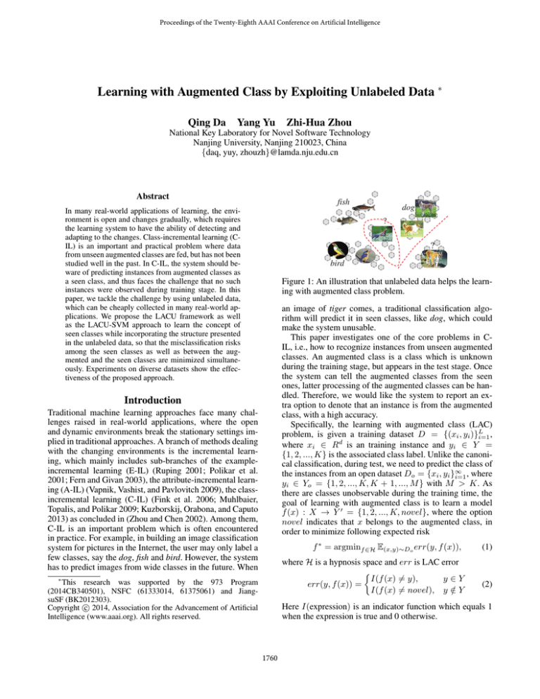
Figure 1: An illustration that unlabeled data helps the learning with augmented class problem.
an image of tiger comes, a traditional classification algorithm will predict it in seen classes, like dog, which could
make the system unusable.
This paper investigates one of the core problems in CIL, i.e., how to recognize instances from unseen augmented
classes. An augmented class is a class which is unknown
during the training stage, but appears in the test stage. Once
the system can tell the augmented classes from the seen
ones, latter processing of the augmented classes can be handled. Therefore, we would like the system to report an extra option to denote that an instance is from the augmented
class, with a high accuracy.
Specifically, the learning with augmented class (LAC)
problem, is given a training dataset D = {(xi , yi )}L
i=1 ,
where xi 2 Rd is an training instance and yi 2 Y =
{1, 2, ..., K} is the associated class label. Unlike the canonical classification, during test, we need to predict the class of
the instances from an open dataset Do = {xi , yi }1
i=1 , where
yi 2 Yo = {1, 2, ..., K, K + 1, ..., M } with M > K. As
there are classes unobservable during the training time, the
goal of learning with augmented class is to learn a model
f (x) : X ! Y 0 = {1, 2, ..., K, novel}, where the option
novel indicates that x belongs to the augmented class, in
order to minimize following expected risk
Introduction
Traditional machine learning approaches face many challenges raised in real-world applications, where the open
and dynamic environments break the stationary settings implied in traditional approaches. A branch of methods dealing
with the changing environments is the incremental learning, which mainly includes sub-branches of the exampleincremental learning (E-IL) (Ruping 2001; Polikar et al.
2001; Fern and Givan 2003), the attribute-incremental learning (A-IL) (Vapnik, Vashist, and Pavlovitch 2009), the classincremental learning (C-IL) (Fink et al. 2006; Muhlbaier,
Topalis, and Polikar 2009; Kuzborskij, Orabona, and Caputo
2013) as concluded in (Zhou and Chen 2002). Among them,
C-IL is an important problem which is often encountered
in practice. For example, in building an image classification
system for pictures in the Internet, the user may only label a
few classes, say the dog, fish and bird. However, the system
has to predict images from wide classes in the future. When
f ⇤ = argminf 2H E(x,y)⇠Do err(y, f (x)),
where H is a hypnosis space and err is LAC error
⇢
I(f (x) 6= y),
y2Y
err(y, f (x)) =
I(f (x) 6= novel), y 2
/Y
⇤
This research was supported by the 973 Program
(2014CB340501), NSFC (61333014, 61375061) and JiangsuSF (BK2012303).
Copyright c 2014, Association for the Advancement of Artificial
Intelligence (www.aaai.org). All rights reserved.
(1)
(2)
Here I(expression) is an indicator function which equals 1
when the expression is true and 0 otherwise.
1760
The main challenge of the task lies under that no instances from augmented classes are observed in the training set. Meanwhile, in many real-world applications a large
amount of unlabeled data can be easily collected. Previous
studies (Chapelle, Schölkopf, and Zien 2006; Zhu and Goldberg 2009; Zhou and Li 2010) have disclosed that unlabeled
data implies useful information that can help improve the
classification performance particularly when the number of
training instances is limited. Inspired from these studies, we
investigate using unlabeled data to help the LAC problem,
where the number of seen classes is limited. Our intuition
is that, as illustrated in Figure 1, when the unlabeled data is
sufficient, large margin classifiers can be identified, which
are usually separators between classes. Therefore the large
margin separators surrounding the seen classes can help distinguish augmented classes.
Following this idea, we present the LACU (Learning with
Augmented Class with Unlabeled data) framework and the
LACU-SVM approach to the learning with augmented class
problem. The proposed method combines the large margin principle from the SVM learning algorithm, with the
low density separator technique from semi-supervised learning algorithms (Chapelle and Zien 2005). By adopting the
one-vs-rest approach, the LACU-SVM picks a classification boundary among all low density separators that minimizes the empirical risk and structure risk as well as the
augment risk simultaneously. An efficient method based on
the concave-convex procedure (CCCP) is applied for solving the optimization problem. Experiments on datasets from
several diverse domains show that the proposed approach
significantly outperforms comparison methods.
The rest of this paper starts with an introduction of the related work. Then the LACU framework is presented, which
is followed by the empirical studies. The paper ends with a
section of discussion and conclusion.
is different with the LAC error. Though one could still use
the rejection methods for learning with augmented class, as
noticed in (Scheirer et al. 2013) that high confidence predictions do not necessarily lead to a small LAC error.
The open set recognition problem is an alternative term
for the LAC problem mainly used by the pattern recognition community. It has been applied in face recognition (Li
and Wechsler 2005), speaker recognition (Reynolds 2002),
etc. Most of these studies are based on simple heuristics.
In (Phillips, Grother, and Micheals 2011), it focuses on the
operating threshold so that an instance is classified to seen
classes only if the confidence is above the threshold. In
(Scheirer et al. 2013), the risk over open space is considered and new decision boundaries are added to minimize the
regions for the seen classes.
The outlier detection problem (Hodge and Austin 2004)
requires to identify abnormal instances from a given data set.
It is possible that outlier detection methods can be used for
the LAC problem by predicting abnormal instances as novel.
However, outlier detection is fundamentally different with
the LAC problem since it relies on the application-specific
definition of outlier, but does not minimize the LAC error.
The class discovery problem tries to find the examples of
the rare classes which are unknown as a prior, but known
to be existent in the training data (Pelleg and Moore 2005;
Hospedales, Gong, and Xiang 2013). The augmented classes
differ from the rare classes mainly in two aspects: First, the
augmented class is not necessarily a rare class, but can become a large class. Second, it is possible to query examples
of a rare class since they are already in the training data,
while it is not possible for the augmented classes since their
examples only appear in the test data.
The LACU Framework
The Framework
Related Work
In many applications, a large amount of unlabeled data can
be easily collected. Thus we may use unlabeled data to help
the LAC problem. Besides the training set, we can access
an unlabeled dataset Du = {xi }L+U
i=L+1 sampled from Do
during the training time.
Based on the successful large margin classifiers, our assumption is that classes, even without been labeled, should
be divided by large margin separators. Therefore, when discriminating one seen class to other seen classes, the unlabeled data can help us identify many large margin separators that have similar performance to the seen classes. Then
to minimize the augment risk, among these separators, we
select the one that is closest to the labeled region.
Denote f (x) 2 H be the classification function, `h (f, D)
be the empirical loss on training examples, `u (f, Du ) be the
loss of in-margin quantity on unlabeled data and `a (f, D) be
the augment loss which supports a decision boundary closer
to the labeled examples. In the LACU framework, we search
for a classifier for the LAC problem by minimizing following objective function
Incremental learning requires the necessary adaption of machine learning methods to the changes of an open and dynamic environment, and class-incremental learning (C-IL)
(Zhou and Chen 2002) is a particularly branch that focuses
on the emerging classes. In (Fink et al. 2006; Kuzborskij,
Orabona, and Caputo 2013), the binary classifiers of each
new class is added incrementally and trained by sharing the
hypothesis of the existing classes. In (Muhlbaier, Topalis,
and Polikar 2009), ensemble method is applied by incrementally introducing base learner trained from data containing new classes. However, these C-IL methods address how
to adapt to augmented classes only when a few of their instances are given, but can not be applied to the LAC problem
as no such instances are available.
The classification with a reject option (Chow 1970) aims
at making reliable prediction by introducing the reject option when the classifier is not confident on the prediction. Loss functions were proposed to incorporate the rejection cost (Bartlett and Wegkamp 2008; Yuan and Wegkamp
2010), where making a wrong prediction could result in an
error with a cost 1 and making a rejection always has a cost
smaller than 1. It is clear that the loss with rejection cost
min kf k2H +C1 `h (f, D)+C2 `u (f, Du )+C3 `a (f, D), (3)
f 2H
1761
Algorithm 1 LACU-SVM Training Algorithm
Input:
D:
Training examples {xi , yi }L
i=1
Du :
Unlabeled data set {xi }L+U
i=L+1
C1 , C2 , , ⌘: Parameters of algorithm
Output:
{✓ k }K
Parameters of learned model
k=1 :
1: for each k 2 {1, ..., K} do
2:
t=0
3:
Let ✓tk be the solution of a standard SVM trained on
Dk = {(xi , yik = 2I(yi = k) 1)|(xi , yi ) 2 D}
4:
Calculate the kernel matrix G
5:
Calculate linear coefficient ⇣ by Eq.(9)
6:
Calculate i and V as
⇢
C2 , yik f (xi |✓tk ) < s and 1  i  L + 2U
=
i
0,
otherwise
where the first term kf k2H measures the complexity of the
classification model, and C1 , C2 , C3 is the coefficients to
balance these losses.
LACU-SVM
Following the one-vs-rest strategy to multi-class classification, we extends the support vector machine (Vapnik 2000)
to the optimization objective in Eq. (3), to obtain the LACUSVM approach. In LACU-SVM, the optimization in Eq.
(3) is applied K times, each treating a seen class as positive (yi = +1) and the rest seen classes as negative ones
(yi = 1) in turn.
Denote f (x) = wT (x) + b be the linear classification
function, `h (f, D) be the hinge loss on labeled data
XL
`h (f, D) =
max(0, 1 yi f (xi )).
i=1
To search for the large margin separator in the unlabeled
data, we use the definition of `u (f, Du ) which can be evaluated by summing up the in-margin quantity as in (Chapelle
and Zien 2005)
XL+U
max(0, 1 |f (xi )|).
`u (f, Du ) =
V = mini2I + yik f (xi |✓tk )
7:
repeat
k
8:
Solve Eq.(8) to obtain ✓t+1
9:
t=t+1
10:
Update i and V as in step 6
11:
until ✓tk = ✓tk 1
12: end for
13: return {✓ k }K
k=1
i=L+1
We define `a (f, D) to control the move of the separator
by adjusting the minimum margin values to minimize the
augment loss as
`a (f, D) = mini2I + yi f (xi )
mini2I yi f (xi ),
Rs (z) = H1 (z) Hs (z), where Hs (z) = max(0, s z).
We then turn to solve the following minimization problem
where I and I are the indices of positive examples and
negative examples in the training data, respectively.
After K classifiers are trained from Eq.(3) with the above
losses, each for an seen class, we use the following prediction rule for a test instance x
+
min J(✓) = J1 (✓) + J2 (✓)
✓
s.t.
ŷ = argmaxk=1,..,K,novel fk (x),
where fnovel ⌘ 0, ties at 0 are predict as novel, and other
ties are broken randomly.
However, the objective function of LACU-SVM in Eq.(3)
is complicated, we thus consider the alternative objective
function kf k2H + C1 `h (f, D) + C2 `u (f, Du ) with an extra
constraint defined as
mini2I + yi f (xi )
mini2I yi 
.
 yj f (xj ), 8j 2 I .
(4)
Even though, the objective function is still overly complex
because of the symmetric hinge loss used in `u (f, Du ).
From the derivation in (Collobert et al. 2006), the symmetric
hinge loss can be approximated by
max(0, 1
mini2I + yi f (xi ) +  yj f (xj ), 8j 2 I
⌘ XL
1 XL+U
1 XL
yi 
f (xi ) 
yi (6)
i=1
i=L+1
i=1
L
U
L
where ✓ = (w, b) is the model parameter, J1 (✓) = kf k2H +
PL+2U
C1 `h (f, D)+C2 i=L+1 H1 (yi f (xi )) is a convex function,
PL+2U
and J2 (✓) = C2 i=L+1 Hs (yi f (xi )) is a concave function. Here yi = +1 for L + 1  i  L + U and yi = 1 for
L + U + 1  i  L + 2U , xL+U +i = xL+i for 1  i  U .
The constraint of Eq.(6) is introduced to avoid classifying
all unlabeled data to one class with a very large margin, by
limiting the fraction of positive data in unlabeled data within
a certain range defined by a parameter ⌘ > 0, since the positive instances always take less fraction in the unlabeled data
than in the labeled data following the one-vs-rest strategy.
After the decomposition of the objective function, the
concave-convex procedure (CCCP) (Yuille and Rangarajan
2003) then can be applied to the optimization problem as in
(Collobert et al. 2006). CCCP is an algorithm which solves
a difference of convex functions programming as a sequence
of convex programming, and is proved to converge with both
convex and non-convex constraints (Lanckriet and Sriperumbudur 2009). In each iteration of CCCP to solve Eq.(5),
we needs to solve following subproblem
Here > 0 is a parameter controlling the degree of how the
decision boundary is close to the positive examples. This
constraint is equivalent to a series of constraints by eliminating one of the min function as
mini2I + yi f (xi ) +
(5)
|z|) ⇡ Rs (z) + Rs ( z) + constant.
Here Rs (z) = min(1
s, max(0, 1
z)) is the ramp
loss with a hyper-parameter s 2 ( 1, 0]. It can be further
rewritten as the difference between two hinge losses, i.e.,
✓t+1 = argmin✓ J1 (✓) + J20 (✓t ) · ✓ ,
1762
(7)
Experiments
where the objective function of the subproblem becomes a
summation of a convex term and a linear term. Note that
there is still a non-convex constraint which involves a min
function as in Eq.(4). To deal with this issue, we combine the alternative optimization technique into the CCCP
framework, i.e., at time t + 1, we use a fixed value V =
mini2I + yi f (xi |✓t ) instead of mini2I + yi f (xi |✓t+1 ). Then
the above optimization of Eq.(7) can be reformulated as dual
form of a quadratic programming problem using standard
SVM techniques as
1 T
↵ G↵
(8)
max↵ ⇣ T ↵
2
s.t. 0  yi ↵i  C1 , 1  i  L
L + 1  i  L + 2U
i  yi ↵i  C2
i,
↵L+2U +1  0, ↵L+2U +2 0
↵i  0,
>
↵ 1=0
Comparison methods
To validate the the effectiveness of LACU-SVM, we conduct
experiments on benchmark datasets from several diverse domains, compared with state-of-the-art methods including:
LOF: Local Outlier Factor (Breunig et al. 2000) is a powerful outlier detector, where the degree of being an outlier
depends on how isolated the object is with respect to the
surrounding neighborhood so that local outliers can also be
detected. We use LOF for detecting augmented class, and
use the predictions of the one-vs-rest SVM for the other
none-outliers. This strategy is also employed for the following outlier detectors.
iForest: iForest (Liu, Ting, and Zhou 2008) is a state-ofthe-art outlier detector which takes advantage of two outliers
quantitative properties, i.e., few and different, by exploring
the concept of isolation of samples.
OC-SVM: One-class SVM (Schölkopf et al. 2001) is another state-of-the-art outlier detector (Ma and Perkins 2003),
which computes a binary function that is supposed to capture
regions in input space where the probability density lives.
MOC-SVM: Since OC-SVM can hardly find local outliers since it essentially seeks for a hyperplane to separate
the data and the origin. Thus, for this comparison method,
we train multiple one-class svms for outlier detection, i.e.,
one OC-SVM for each seen class.
1-vs-Set: 1-vs-Set Machine (Scheirer et al. 2013) considers the risk over open space by introducing extra decision
boundaries to minimize the regions for the seen classes.
OVR-SVM: One-vs-rest SVM is a powerful scheme for
multi-class classification (Rifkin and Klautau 2004). In the
original OVR-SVM, a test instance x is predicted as class y
if y = argmaxk=1,2,..,K fk (x) where fk is the binary SVM
for class k. To adapt OVR-SVM for predicting the augmented class, we let the model return the class y only when
maxk fk (x) > 0, otherwise return the augmented class.
In the experiments, we use the implementations of OVRSVM, OC-SVM and MOC-SVM in the LIBSVM software
(Chang and Lin 2011), and the implementations of 1-vs-Set
Machine and iForest from the code released by the corresponding authors. The coefficient C in SVM is selected via
cross validation on training data using the original OVRSVM. The width for Gaussian kernel is set to a fixed value
of 1/d. For LOF, the minimum and maximum number of
neighbors are 3 and 9, respectively. Note that the original
LOF does not have a kernel version, so we replace the Euclid distance de with 1 exp( de ) for Gaussian kernel.
Since such adaption can not be applied for iForest, we use
the same version of iForest with the default parameters in its
R-pacakge for both kernels. For LACU-SVM, s in the ramp
loss is set to 0.3, C1 is set to C, C2 is set to C1 L/U , and
number of iterations is set to 10 for all experiments. Without further explanation, the parameters ⌘ and in LACUSVM are set to 1.3 and 0.1 respectively by default. For evaluation, we focus on the macro-averaged F1 by treating the
augmented class as the (K + 1)-th class, to eliminate the
influence of unbalanced data.
L + 2U + 3  i  L + 2U + 2 + |I |
where N = L + 2U + 2 + |I | is the total number of dual
variables. i is C2 for yi f (xi |✓t ) < s (L + 1  i  L +
2U ), 0 otherwise. G 2 RN ⇥N is the kernel matrix where
Gij = h (xi ), (xi )i. Besides the already defined L + 2U
instances, here we introduce another (2 + |I |) instances,
PL+U
where (xL+2U +1 ) = (xL+2U +2 ) = U1 i=L+1 (xi )
and xi = x[I ]i L 2U 2 for L + 2U + 3  i  N . The
linear coefficient of dual variable is
8
>
yi ,
>
>
< 1 PL
i=1 yi ,
⇣i = L
⌘ PL
>
y,
>
> L i=1 i
:
V
,
1  i  L + 2U
(9)
i = L + 2U + 1
i = L + 2U + 2
L + 2U + 3  i  L + 2U + 2 + |I |
This is a quadratic programming (QP) problem very close
to the standard SVM dual problem and can be efficiently
solved using the existing Sequential Minimal Optimization
(SMO) solver (Bottou and Lin 2007). The final optimal solution is given by
XN
w=
↵i (xi ),
i=1
and b can be obtained by the KKT condition, i.e., yi (wT x +
b) = 1, for 0 < yi ↵i < C1 (1  i  L) or
i < yi ↵ i <
C2
(L
+
1

i

L
+
2U
).
i
The overall description of the proposed method is presented in Algorithm 1. The method takes labeled training
dataset D, unlabeled dataset Du and the four parameters C1 ,
C2 , , ⌘ as input. It trains K binary classifiers for each seen
class following the one-vs-rest strategy in the outer iteration. For each seen class k 2 {1, ..., K}, LACU-SVM initializes the ✓0k as the solution to the standard SVM trained
on labeled data Dk only as in line 3, and then calculates the
coefficients of Eq.(8), i.e., G, ⇣, and V as in line 4, 5
and 6. Then it starts the iteration of CCCP by solving the
quadratic programming problem in Eq.(8) from line 7 to 11.
In each inner iteration, it only requires solving a QP problem by SMO in line 8, and in our empirical study we find
that it usually converges only after a few iterations, making
the training procedure for each class roughly enjoy the computational complexity of SMO.
1763
2,
4,
5,
7,
9
3,
5,
6,
7,
9
1,
2,
4,
5,
6
0,
3,
6,
7,
9
0,
3,
5,
6,
8
1,
3,
4,
5,
6
1,
3,
6,
7,
8
0,
2,
5,
6,
7
0,
2,
3,
7,
9
0,
1,
2,
3,
6
2,
4,
5,
7,
9
3,
5,
6,
7,
9
1,
2,
4,
5,
6
0,
3,
6,
7,
9
0,
3,
5,
6,
8
1,
3,
4,
5,
6
1,
3,
6,
7,
8
0,
2,
5,
6,
7
0,
2,
3,
7,
9
0,
1,
2,
3,
6
Figure 2: Comparisons of different methods on MNIST dataset (linear kernel)
Figure 3: Comparisons of different methods on MNIST dataset (Gaussian kernel)
Results
test instances
Handwritten Digit Image Classification In the first experiment, we conducted experiments on the MNIST handwritten digit dataset, where 5 classes are randomly selected as
seen classes from the all the 10 classes. The number of training data, unlabeled data and test data are 500, 500 and 1000.
For each configuration (with different seen classes), the experiments are repeated for 10 times and both the mean and
the standard variance of the performance are reported. The
results of 10 randomly selected configurations are shown in
Figure 2/3 and for linear/Gaussian kernel. For linear kernel,
the 1-vs-set machine shows to outperform OVR-SVM in all
cases and the LOF methods outperforms OVR-SVM in near
50% cases, while LACU-SVM always obtains the highest
performance and is significantly better than the compared
methods. For Gaussian kernel, LACU-SVM also achieves
the best performance, while the OVR-SVM is slightly worse
and significantly better than the other five methods. In both
kernels, the outlier detection methods with iForest, OCSVM and MOC-SVM produce the worst performance.
To further verify the effectiveness of LACU-SVM, we
show some demonstrations of test images for the first configuration in Figure 4. The images are from unseen classes.
LACU-SVM successfully identifies the novelty, while OVRSVM predicts them to be seen classes. It is not surprising that OVR-SVM makes the wrong decisions since those
samples are very similar to the seen classes and OVR-SVM
never observes them during training. At the other hand, by
exploiting the unlabeled data, the proposed LACU-SVM
successfully recognizes these images as augmented classes.
Document Classification In the second experiment, we
conduct experiments on the popular text dataset, i.e., 20
Newsgroups, to show some statistical results of all methods over various configurations. This dataset consists of
documents from 20 different topics. Some of these topics are highly related like comp.sys.ibm.pc.hardware and
predictions
OVR-SVM
novel
novel
novel
novel
novel
Figure 4: Examples of predictions made by OVR-SVM and
LACU-SVM. The classes of 0,1,2,3,6 are observed in training set, and all classes are in the test set.
comp.sys.mac.hardware, which will be an issue, when one
belongs to seen classes and the other one does not. We also
limit the number of seen classes to 5. The number of training data, unlabeled data and test data are 500, 1000 and 1000
respectively. We randomly sample 100 configurations from
all possible combinations, and for each configuration the experiment is repeated for 10 times. The results of win/tie/loss
counts of all possible pairs of methods are shown in Table
1, for both linear and Gaussian kernel. The number in the
ith row and the jth column denotes the times of win, tie and
loss of the method in the corresponding row, versus that in
the corresponding column, over all the 100 configurations.
The detailed results of the macro-averaged F1 performances
will be presented in the longer version of the paper.
It shows that, the proposed LACU-SVM wins all the configurations compared with the four outlier detection methods, and significantly outperforms the OVR-SVM and 1-vsSet machine with the loss rate at most 7% for both linear
and Gaussian kernels. Besides our method, OVR-SVM wins
most comparisons, even has beaten 1-vs-Set machine in 74%
case with linear kernel and 100% cases with Gaussian kernel, which implies that it maybe inappropriate to simply in-
1764
Table 1: The results of win/tie/loss information with 100 randomly selected configurations on 20 Newsgroup dataset (paired
two-tailed t-test at 95% significance level)
Method
Linear kernel
LOF
LOF
-
iForest
0/100/0
OC-SVM
Gaussian kernel
iForest OC-SVM MOC-SVM 1-vs-Set OVR-SVM LACU-SVM
0/100/0 0/0/100
-
100/0/0 100/0/0
LOF
iForest OC-SVM MOC-SVM 1-vs-Set OVR-SVM LACU-SVM
0/7/93
0/0/100
0/0/100
0/0/100
-
0/0/100
0/7/93
0/0/100
0/0/100
0/0/100
0/100/0
-
72/28/0
0/0/100
0/0/100
0/0/100
69/31/0 69/31/0
-
0/0/100
0/0/100
0/0/100
100/0/0
-
0/26/74
100/0/0
74/26/0
100/0/0
84/15/1
MOC-SVM 93/7/0 93/7/0 0/28/72
1-vs-Set 100/0/0 100/0/0 100/0/0
OVR-SVM 100/0/0 100/0/0 100/0/0
LACU-SVM 100/0/0 100/0/0 100/0/0
0/0/100
0/0/100
0/0/100
0/0/100
0/31/69
0/0/100
0/0/100
0/0/100
0/0/100
-
0/42/58
0/0/100
0/0/100
0/0/100
100/0/0 100/0/0 58/42/0
-
0/1/99
0/0/100
0/0/100
1/15/84
100/0/0 100/0/0 100/0/0
99/1/0
-
0/0/100
0/4/96
-
7/15/78
100/0/0 100/0/0 100/0/0
100/0/0
100/0/0
-
7/18/75
78/15/7
-
100/0/0 100/0/0 100/0/0
100/0/0
96/4/0
75/18/7
-
troducing an extra parallel decision boundary to limit the
positive region as in 1-vs-Set when the labeled examples of
each seen class may not be distributed in a very concentrative region. The outlier detection methods nearly lose all the
comparisons, especially for LOF and iForest which predict
almost all test instances as none-outliers. It is possibly because outliers are usually decided by specific tasks, and outlier detection does not minimize the LAC error.
Object Recognition In the last experiment, we conduct the experiment on the object recognition task, i.e., the
Caltech101 dataset (Fei-Fei, Fergus, and Perona 2007) (101
classes), to show the performance of different methods when
LAC problem becomes more challenging (with more unseen
classes). We limit the number of seen classes to 5 and let the
number of test classes (M ) vary form 30 to 100 . The number of training images for each seen classes is set to 20 as
a popular setting. The number of unlabeled images and test
images for each test classes are set to 5 and 10 respectively.
We extract the spatial histograms of visual words with 3600
dimensions for each image. We only report the results with
linear kernel since it is considered to be more appropriate for
such representation. For different number of test classes, we
randomly sample 200 configurations and for each configuration the experiment is repeated for 5 times. The overall mean
of macro-average F1 is reported in Figure 5.
It shows that, with the increasing number of test classes,
the performance of most methods degrade as expected.
Among all the methods, LACU-SVM achieves the best performance. The 1-vs-set machine does not achieve a comparable performance. All the outlier detection methods fail in
this data, which further indicates the instances from unseen
classes should not be simply regarded as outliers when dealing with LAC problem.
We further investigate the influence of different parameters in LACU-SVM, i.e., ⌘ and , in Figure 6(a) and Figure
6(b) respectively. We let ⌘ vary from 1.1 to 1.5 with an interval of 0.5 and let vary from 0.05 to 0.45 with an interval
of 0.05. The performance tendencies with different number
of test classes are also studied, with M = 40, 60, 80, 100,
for an unbiased analysis of the influence of parameters. The
results show that, the performance of LACU-SVM is overall
not very sensitive to the parameters, and only with a small
M , the performance trends to increase with a larger ⌘ as well
as a smaller . For M > 40, there is no significant difference
between the performance produced by various parameters.
0/100/0 0/31/69
-
Figure 5: Performance with different number of test classes
on Caltech101 dataset
(a) With different ⌘
(b) With different
Figure 6: The influence of parameters ⌘ and in LACUSVM on Caltech101 dataset
Conclusion
Learning with augmented class is a very practical problem
when a system needs to predict the data from an unlimited source. In this paper, we propose to tackle the problem
with the help of unlabeled data. The experiments on several
datasets show the effectiveness of the proposed method. In
the future work, there are several important issues to be considered. One is that, besides the current SVM based method,
we would like to apply more state-of-the-art multi-class algorithms to the LACU framework. Developing a theoretical
grounded method for the LAC problem is also of interest.
Acknowledgements: We want to thank anonymous reviewers for comments and suggestions, and Yu-Feng Li, DeChuan Zhan for discussions and reading the draft.
References
Bartlett, P. L., and Wegkamp, M. H. 2008. Classification
with a reject option using a hinge loss. Journal of Machine
Learning Research 9:1823–1840.
1765
Muhlbaier, M.; Topalis, A.; and Polikar, R. 2009. Learn++
nc: Combining ensemble of classifiers with dynamically
weighted consult-and-vote for efficient incremental learning
of new classes. IEEE Trans. Neural Networks 20(1):152–
168.
Pelleg, D., and Moore, A. W. 2005. Active learning for
anomaly and rare-category detection. In Advances in Neural
Information Processing Systems 17. 1073–1080.
Phillips, P. J.; Grother, P.; and Micheals, R. 2011. Evaluation
methods in face recognition. In Li, S. Z., and Jain, A. K.,
eds., Handbook of Face Recognition. New York: Springer.
329–348.
Polikar, R.; Upda, L.; Upda, S.; and Honavar, V. 2001.
Learn++: An incremental learning algorithm for supervised
neural networks. IEEE Trans. Systems, Man, and Cybernetics, Part C 31(4):497–508.
Reynolds, D. A. 2002. An overview of automatic speaker
recognition technology. In Proceedings of the International
Conference on Acoustics, Speech, and Signal Processing,
4072–4075.
Rifkin, R., and Klautau, A. 2004. In defense of one-vsall classification. Journal of Machine Learning Research
5:101–141.
Ruping, S. 2001. Incremental learning with support vector machines. In Proceedings of the 1st IEEE International
Conference on Data Mining, 641–642.
Scheirer, W.; de Rezende Rocha, A.; Sapkota, A.; and Boult,
T. 2013. Toward open set recognition. IEEE Trans. Pattern
Analysis and Machine Intelligence 35(7):1757–1772.
Schölkopf, B.; Platt, J. C.; Shawe-Taylor, J.; Smola, A. J.;
and Williamson, R. C. 2001. Estimating the support
of a high-dimensional distribution. Neural Computation
13(7):1443–1471.
Vapnik, V.; Vashist, A.; and Pavlovitch, N. 2009. Learning
using hidden information (learning with teacher). In Proceedings of International Joint Conference on Neural Networks, 3188–3195.
Vapnik, V. 2000. The Nature of Statistical Learning Theory.
New York: Springer Verlag.
Yuan, M., and Wegkamp, M. 2010. Classification methods
with reject option based on convex risk minimization. Journal of Machine Learning Research 11:111–130.
Yuille, A. L., and Rangarajan, A. 2003. The concave-convex
procedure. Neural Computation 15(4):915–936.
Zhou, Z.-H., and Chen, Z.-Q. 2002. Hybrid decision tree.
Knowledge-Based Systems 15(8):515–528.
Zhou, Z.-H., and Li, M. 2010. Semi-supervised learning by disagreement. Knowledge and Information Systems
24(3):415–439.
Zhu, X., and Goldberg, A. B. 2009. Introduction to SemiSupervised Learning. San Rafael, Argentina: Morgan &
Claypool.
Bottou, L., and Lin, C.-J. 2007. Support vector machine
solvers. In Bottou, L.; Chapelle, O.; DeCoste, D.; and Weston, J., eds., Large Scale Kernel Machines. Cambridge,
MA: MIT Press. 301–320.
Breunig, M. M.; Kriegel, H.-P.; Ng, R. T.; and Sander, J.
2000. LOF: Identifying density-based local outliers. ACM
SIGMOD Record 29(2):93–104.
Chang, C., and Lin, C. 2011. LIBSVM: A library for support vector machines. ACM Trans. Intelligent Systems and
Technology 2(3):27.
Chapelle, O., and Zien, A. 2005. Semi-supervised classification by low density separation. In Proceedings of the 10th
International Workshop on Artificial Intelligence and Statistics, 57–64.
Chapelle, O.; Schölkopf, B.; and Zien, A. 2006. SemiSupervised Learning. Cambridge, MA: MIT press.
Chow, C. 1970. On optimum recognition error and reject
tradeoff. IEEE Trans. Information Theory 16(1):41–46.
Collobert, R.; Sinz, F.; Weston, J.; and Bottou, L. 2006.
Large scale transductive SVMs. Journal of Machine Learning Research 7:1687–1712.
Fei-Fei, L.; Fergus, R.; and Perona, P. 2007. Learning generative visual models from few training examples: An incremental bayesian approach tested on 101 object categories.
Computer Vision and Image Understanding 106(1):59–70.
Fern, A., and Givan, R. 2003. Online ensemble learning: An
empirical study. Machine Learning 53(1-2):71–109.
Fink, M.; Shalev-Shwartz, S.; Singer, Y.; and Ullman, S.
2006. Online multiclass learning by interclass hypothesis
sharing. In Proceedings of the 23rd International Conference on Machine Learning, 313–320.
Hodge, V. J., and Austin, J. 2004. A survey of outlier detection methodologies. Artificial Intelligence Review 22(2):85–
126.
Hospedales, T. M.; Gong, S.; and Xiang, T. 2013. Finding
rare classes: Active learning with generative and discriminative models. IEEE Trans. Knowledge and Data Engineering
25(2):374–386.
Kuzborskij, I.; Orabona, F.; and Caputo, B. 2013. From n to
n+1: Multiclass transfer incremental learning. In Proceedings of the 26th IEEE Conference on Computer Vision and
Pattern Recognition, 3358–3365.
Lanckriet, G. R., and Sriperumbudur, B. K. 2009. On the
convergence of the concave-convex procedure. In Advances
in Neural Information Processing Systems 22. 1759–1767.
Li, F., and Wechsler, H. 2005. Open set face recognition using transduction. IEEE Trans. Pattern Analysis and Machine
Intelligence 27(11):1686–1697.
Liu, F. T.; Ting, K. M.; and Zhou, Z.-H. 2008. Isolation
forest. In Proceedings of the 8th IEEE International Conference on Data Mining, 413–422.
Ma, J., and Perkins, S. 2003. Time-series novelty detection
using one-class support vector machines. In Proceedings
of the International Joint Conference on Neural Networks,
1741–1745.
1766