Proceedings of the Twenty-Ninth AAAI Conference on Artificial Intelligence
Tensor-Variate Restricted Boltzmann Machines
Tu Dinh Nguyen†, Truyen Tran†‡, Dinh Phung†, Svetha Venkatesh†
†Center for Pattern Recognition and Data Analytics
School of Information Technology, Deakin University, Geelong, Australia
‡Institute for Multi-Sensor Processing and Content Analysis
Curtin University, Australia
{ngtu,truyen.tran,dinh.phung,svetha.venkatesh}@deakin.edu.au
Abstract
Restricted Boltzmann Machines (RBMs) are an important
class of latent variable models for representing vector data.
An under-explored area is multimode data, where each data
point is a matrix or a tensor. Standard RBMs applying to such
data would require vectorizing matrices and tensors, thus resulting in unnecessarily high dimensionality and at the same
time, destroying the inherent higher-order interaction structures. This paper introduces Tensor-variate Restricted Boltzmann Machines (TvRBMs) which generalize RBMs to capture the multiplicative interaction between data modes and
the latent variables. TvRBMs are highly compact in that the
number of free parameters grows only linear with the number
of modes. We demonstrate the capacity of TvRBMs on three
real-world applications: handwritten digit classification, face
recognition and EEG-based alcoholic diagnosis. The learnt
features of the model are more discriminative than the rivals,
resulting in better classification performance.
1
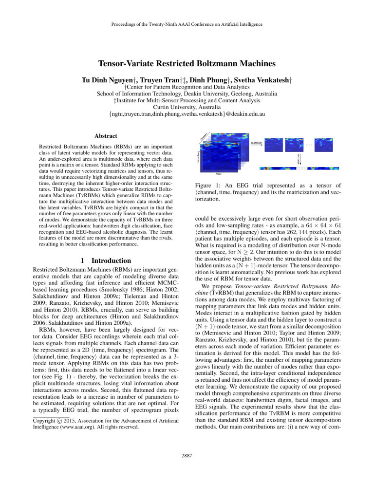
Figure 1: An EEG trial represented as a tensor of
hchannel, time, frequencyi and its the matricization and vectorization.
could be excessively large even for short observation periods and low-sampling rates - as example, a 64 × 64 × 64
hchannel, time, frequencyi tensor has 262, 144 pixels). Each
patient has multiple episodes, and each episode is a tensor.
What is required is a modeling of distribution over N-mode
tensor space, for N ≥ 2. Our intuition to do this is to model
the associative weights between the structured data and the
hidden units as a (N + 1)-mode tensor. The tensor decomposition is learnt automatically. No previous work has explored
the use of RBM for tensor data.
We propose Tensor-variate Restricted Boltzmann Machine (TvRBM) that generalizes the RBM to capture interactions among data modes. We employ multiway factoring of
mapping parameters that link data modes and hidden units.
Modes interact in a multiplicative fashion gated by hidden
units. Using a tensor data and the hidden layer to construct a
(N + 1)-mode tensor, we start from a similar decomposition
to (Memisevic and Hinton 2010; Taylor and Hinton 2009;
Ranzato, Krizhevsky, and Hinton 2010), but tie the parameters across each mode of variation. Efficient parameter estimation is derived for this model. This model has the following advantages: first, the number of mapping parameters
grows linearly with the number of modes rather than exponentially. Second, the intra-layer conditional independence
is retained and thus not affect the efficiency of model parameter learning. We demonstrate the capacity of our proposed
model through comprehensive experiments on three diverse
real-world datasets: handwritten digits, facial images, and
EEG signals. The experimental results show that the classification performance of the TvRBM is more competitive
than the standard RBM and existing tensor decomposition
methods. Our main contributions are: (i) a new way of com-
Introduction
Restricted Boltzmann Machines (RBMs) are important generative models that are capable of modeling diverse data
types and affording fast inference and efficient MCMCbased learning procedures (Smolensky 1986; Hinton 2002;
Salakhutdinov and Hinton 2009c; Tieleman and Hinton
2009; Ranzato, Krizhevsky, and Hinton 2010; Memisevic
and Hinton 2010). RBMs, crucially, can serve as building
blocks for deep architectures (Hinton and Salakhutdinov
2006; Salakhutdinov and Hinton 2009a).
RBMs, however, have been largely designed for vector data. Consider EEG recordings wherein each trial collects signals from multiple channels. Each channel data can
be represented as a 2D htime, frequencyi spectrogram. The
hchannel, time, frequencyi data can be represented as a 3mode tensor. Applying RBMs on this data has two problems: first, this data needs to be flattened into a linear vector (see Fig. 1) - thereby, the vectorization breaks the explicit multimode structures, losing vital information about
interactions across modes. Second, this flattened data representation leads to a increase in number of parameters to
be estimated, requiring solutions that are not optimal. For
a typically EEG trial, the number of spectrogram pixels
Copyright c 2015, Association for the Advancement of Artificial
Intelligence (www.aaai.org). All rights reserved.
2887
puting distribution over tensor space using RBM and (ii) a
comprehensive evaluation of the effectiveness of our method
on three applications: handwritten digit classification, face
recognition and alcoholic diagnosis using EEG signals.
The rest of paper is organized as follows. Sec. 2 presents
an insightful review of the related literature. We then describe the standard RBM and tensor notations in Sec. 3, followed by the model presentation and parameter learning of
our Tensor-variate RBM in Sec. 4. The experimental results
on three applications are then reported in Sec. 5. Finally,
Sec. 6 concludes the paper.
2
Figure 2: Graphical illustrations of RBM (left) and TvRBM
(right). The cubic nodes are observed, the sphere nodes are
latent. The TvRBM models the 3D input data of 2 × 4 × 3
and the triangular pyramids represent 4-way factors.
Related Work
The multiway data modeling problem is well-studied. The
most popular approach is to treat the entire dataset as a (N +
1)-mode tensor and apply tensor decomposition methods.
Two most well-known techniques are the Tucker decomposition (Tucker 1963) and PARAFAC (Carroll and Chang
1970). More recently, variants have been introduced, including 2D nonnegative matrix factorization (2DNMF) (Zhang,
Chen, and hua Zhou 2005), nonnegative Tucker decomposition (Kim and Choi 2007), and nonnegative tensor factorization (Shashua and Hazan 2005). These are linear and do
not generalize to unseen data because data distribution is not
modeled. When seeing a new data point, these methods must
perform an expensive “fold-in” procedure to estimate projection. Probabilistic interpretation has subsequently been
introduced, notably the probabilistic Tucker decomposition
(Chu and Ghahramani 2009) and its nonparametric Bayesian
extension (Xu, Yan, and Qi 2012). These models are directed
whilst the TvRBM is undirected with log-linear parameterization.
For data points in the matrix form (e.g., 2D images), wellknown methods include 2D principal components analysis
(2DPCA) (Yang et al. 2004) and 2D linear discriminant analysis (2DLDA) (Ye, Janardan, and Li 2004). These are also
linear methods with strong assumptions of Gaussian noise.
By contrast, our TvRBM is a probabilistic model that learns
a probabilistic non-linear mapping from data to the representation space. More closely related to the generative nature of
the RBM is factor analysis (FA), which is a directed model
of vector data. Matrix and tensor extensions have been introduced in recent years: matrix-variate FA (MVFA) (Xie et
al. 2008), and the tensor analyzer (Tang, Salakhutdinov, and
Hinton 2013).
Multiplicative interactions and multiway factoring have
been studied within the RBM community to capture the
pairwise association between vectors and the gating effect
(Memisevic and Hinton 2010; Taylor and Hinton 2009;
Ranzato, Krizhevsky, and Hinton 2010), as well as factors
of variation (Reed and Lee 2013). Although the mathematics of decomposing the (N + 1)-order mapping tensor W
between their work and ours has similar tensor factorization
form, the nature of data and the purposes are entirely different. They examine the Cartesian product of two vectors, but
the input data is still vector, not tensor and there does not
exist the concept of “data mode” (e.g., channel, time, frequency). More specially, the pairwise interaction between
pixel elements is considered in (Ranzato, Krizhevsky, and
Hinton 2010), but the pixels are represented as a vector. In
(Memisevic and Hinton 2007; 2010), the transformation between two image vectors is studied, but two similar vectors
do not constitute two orthogonal modes such as time and
frequency. Second, generalizing pairwise transformation to
three or more vectors proves to be difficult. On the other
hand, we study the data in a high-order tensor of orthogonal
modes. The (N+1)-order tensor factorization in our case reveals the structure of the interaction among N modes, while
it is the higher-order interaction between vector elements in
previous work.
3
3.1
Preliminaries
Representing vector data using RBM
Denote by v = (v1 , v2 , ..., vM ) the variable representing the visible data. Our goal is to learn a higher, laK
tent representation h = (h1 , h2 , ..., hK ) ∈ {0, 1} . A
Restricted Boltzmann Machine (RBM) (Smolensky 1986;
Hinton and Salakhutdinov 2006) is a bipartite undirected
graphical model encoding these two layers (see Fig. 2 (left)
for a graphical illustration). The RBM assigns energy for a
joint configuration (v, h) as:
E (v, h; ψ) = − F (v) + a> v + b> h + v> Wh (1)
where a ∈ RM , b ∈ RK are the biases, W ∈ RM×K is
the mapping parameters, and F (v) is type-specific function
P 2
(e.g., F (v) = 0 for binary input and F (v) = −0.5 m vm
for Gaussian variables). The model admits the Boltzmann
distribution: p (v, h; ψ) ∝ exp [−E (v, h; ψ)], where ψ =
{a, b, W} is model parameter.
The bipartite structure of RBM enables units in one layer
become conditionally independent given the other layer.
Thus the conditional distributions over hidden and visible
units are factorized as:
p (v | h; ψ) =
M
Y
p (vm | h)
m=1
p (h | v; ψ) =
K
Y
k=1
2888
p (hk | v)
These provide fast layer-wise MCMC sampling, leading to
efficient stochastic gradient learning, such as Contrastive Divergence (Hinton 2002) and its variant (Tieleman and Hinton 2009).
2009c), and mixed types (Tran, Phung, and Venkatesh 2013)
is omitted. Let:
h
i>
D2 ¯
DN
1 ¯
¯ 1 1D
¯
Gd1 d2 ...dN (h) = W ×
h
d1 ×2 1d2 ×3 ...×N 1dN
3.2
• For binary input, we have F (V ) = 0 (in Eq. (2)) and the
following generative distribution:
Tensor notations
Following (Kolda and Bader 2009), we use plain lowercase letters (e.g., t) to indicate scalar values; bold lowercase letters (e.g., t) for vectors; bold uppercase letters for
matrices (e.g., T); Euler script letters for higher-order tensor, e.g. the N-mode tensor: T ∈ RD1:N where D1:N ,
D1 × D2 × ... × DN is the product space over N dimensions.
Denote by t·i the i-th column vector of matrix T. The symbol “◦” denotes the vector outer product, e.g., the rank-one
N-mode tensor can be written as the outer product of N vectors:
T = x(1) ◦ x(2) ◦ ... ◦ x(N)
¯ n indicate the n-th mode product which is the multiLet ×
plication of a vector with a tensor along mode n, resulting in
a (N − 1)-mode tensor:
p (vd1 d2 ...dN = 1 | h) = σ [ad1 d2 ...dN + Gd1 d2 ...dN (h)]
• For Gaussian input, assuming unit variance, i.e., F (V ) =
−0.5 hV , V i, the generative distribution reads
p(vd1 d2 ...dN |h)=N {ad1 d2 ...dN +Gd1 d2 ...dN (h)};1D1:N
in which 1D1:N is the tensor where all elements are 1.
Once all parameters are fully specified, the new representation of an input data can be obtained
by projecting
onto hidden space ĥ = ĥ1 , ĥ2 , ..., ĥK , where ĥk =
p (hk = 1 | V ) as in Eq. (3). The higher representation can
be used as input for further classification tasks.
¯n t
X =T ×
4.2
where t ∈ RDn , X ∈ RD¬n and D¬n , D{1:N}\n denotes
the product space over N dimensions excluding Dn .
The inner product of two same-sized tensors X , Y ∈ RD1:N
is the sum of their element-wised products:
hX , Y i =
D2
D1 X
X
d1 =1 d2 =1
4
...
DN
X
A major problem with the parameterization in Eq. (2) is the
excessively large number of free parameters which scales
as the product of data mode and hidden dimensions. Q
In particular, the (N + 1)-mode mapping tensor W has K n Dn
elements, which quickly reaches billions when the mode dimensionalities K, D1:N and N are moderate. This makes
learning extremely difficult for several reasons. First, it
would require a large dataset for a robust estimate of parameters. Second, it is hard to control the bounding of hidden ac¯ N+1 1K
tivation values V , W ×
k in Eq. (3). Thus the hidden
posteriors are easily collapsed into either 0 or 1 and no
Q more
learning occurs. Finally, the model requires O K n Dn
memory for parameters.
To this end, we employ (N + 1)-way factoring (Memisevic and Hinton 2010) to construct the multiplicative interactions between visible modes and hidden units. With F
factors, the parameter tensor W is decomposed using the
Kruskal operator as follows:
xd1 d2 ...dN yd1 d2 ...dN
dN =1
Tensor-variate Restricted Boltzmann
Machines
We now describe the Tensor-variate RBM (TvRBM) for
multimode data. See Fig. 2 (right) for an example of TvRBM
to model 3D data.
4.1
(N+1)-way factoring of multiplicative
interactions
Model definition
In TvRBM, the set of visible units is represented by a Nmode tensor V ∈ RD1:N and the hidden units are the same as
in RBM. The goal is to model the joint distribution p(V , h).
The energy in Eq. (1) turns into the following form:
¯ N+1 hi (2)
E(V ,h)=− F(V )+hA ,V i+b> h+hV ,W ×
W = Jλ; W(1) , ..., W(N) , Wh K
=
where F (V ) is type-specific function, A ∈ RD1:N are visible biases, and W ∈ RD1:N ×K are mapping parameters. The
hidden posterior is
¯ N+1 1K
p (hk = 1 | V ) = σ bk + V , W ×
(3)
k
F
X
f=1
(1)
(N)
λf w·f ◦ ... ◦ w·f ◦ w·hf
where λ ∈ RF is the scaling vector, the matrix W(n) ∈
RDn ×F represents the mode-factor weights, and Wh ∈
RK×F the hidden-factor. Here we fix λ = 1 for simplicity,
so we obtain:
where 1K
k is one-hot representation of K-length vector with
−1
all zeros but 1 at k th position, σ (x) = (1 + e−x )
is
the sigmoid function. The generative distribution p (V | h),
on the other hand, is type-specific. In what follows, we
present the most popular cases, namely the binary and Gaussian inputs, but the generalization to Poisson (Salakhutdinov
and Hinton 2009b), multinomial (Salakhutdinov and Hinton
wd1 d2 ...dN k =
F
X
X
(1)
(N)
h
wd1 f ...wdN f wkf
f=1 d1 d2 ...dN k
This factoring allows multiplicative interactions between
modes to be moderated by the hidden units through the
hidden-factor matrix Wh . Thus the model captures the
2889
modes of variation through the new representation by
h. The number P
of mapping parameters is drastically reduced to F (K + n Dn ), which grows linearly rather than
exponentially in N. The memory space requirement decreases accordingly. Importantly, the presence of the decomposition does not lead to chicken-and-egg problem that
can make learning and inference difficult. More specifically, the conditional independence among intra-layer variQK
ables, i.e., p (h | V ) = k=1 p (hk | V ) and p (V | h) =
Q QDn
dn =1 p (vd1 d2 ...dN | h), are not affected. Therefore the
n
proposed model preserves fast sampling and inference properties of RBM.
4.3
However, there are no explicit connection weights between
hidden units and visible ones in the TvRBM. We estimate
these weights from the multiplicative interactions. Assuming that the spatial features lie at n-th mode of the data, the
learnt filters are matrix R given by:
R=
f=1
5
Denote by φ = A , b, W(1) , W(2) ..., W(N) , Wh the
model parameters. Learning seeks the
Pmaximizer of the data
likelihood: L (V ; φ) = p (V ; φ) = h p (V , h; φ) with respect to the parameter φ. The gradient of the log-likelihood
is the difference of two expectations:
(4)
Implementation and Results
In this section, we evaluate the Tensor-variate RBM on three
real-world applications of very different natures: handwritten digit classification, face recognition and alcoholic diagnosis from EEG signals. Our main goal is to demonstrate
the power of TvRBM in learning robust representations for
high-dimensional data with several modes of variation and
limited number of training samples.
∂E (V , h)
∂E (V , h)
∂
log L (V ; φ) = EV ,h
− Eh|V
∂φ
∂φ
∂φ
5.1
where EV ,h is the model expectation w.r.t. p (V , h) and
Eh|V is the data expectation w.r.t. p (h | V ). The data expectation can be computed efficiently using Eq. (3) whilst
the model expectation is intractable due to the sum over
exponential space of hidden units. Fortunately, the Contrastive Divergence procedure (Hinton 2002) allows fast approximation using short Markov chains. Starting from observed data, the
by alternating be chains
collect samples
tween V̂ ∼ P V | ĥ and ĥ ∼ P h | V̂ .
The derivatives with respect to mode- and hidden-factor
matrices are:
∂
E (V , h; φ) = − h> w·hf hX , Y i
(n)
∂wdn f
E
D
∂
(N)
(1)
E
(V
,
h;
φ)
=
−h
◦
...
◦
w
V
,
w
k
h
·f
·f
∂wkf
Implementation
We use binary visible units for image data and Gaussian
ones for EEG signals. Following (Hinton and Salakhutdinov
2006), the pixel intensities of images are normalized into the
range [0, 1] and treated as empirical probabilities of the input.
As factors interact in a multiplicative manner leading to a
potential numerical instability in gradient, a sensible parameter initialization and control of step size in parameter update would stabilize the learning and achieve faster convergence. The factorized parameters are initialized randomly
from N (0; 0.1). We initialize the visible biases using the
first moment matching:
¯ N+1 h0
log V̄ − log 1 − V̄ − W ×
A =
if v ∈ {0, 1}
¯ N+1 h0
V̄ − W ×
if v ∈ R
where h0 is drawn randomly, and V̄ is the mean of the input over the dataset. The hidden bias is initialized as bk =
¯ N+1 1K
− V̄ , W ×
k . For binary models, the step size of is
fixed to 0.01. Hidden, visible and mode-factor learning rates
are fixed to 0.1. In the Gaussian models, the step size and
learning rates are 10 times smaller due to unbounded visible variables. The number of factors F of TvRBM is set to
100. For both RBM and TvRBM, 500 hidden units are used
for images and 200 for EEG signals. Hyperparameters are
specified using cross-validation. We update parameters after seeing “mini-batches” of B = 50 samples. Learning is
terminated after 100 scans through the whole data.
We perform classifications to verify the capability of our
model. Whenever suitable, the classification errors are compared with the results of standard RBM, matrix methods
– 2DPCA (Yang et al. 2004) and 2DNMF (Zhang, Chen,
and hua Zhou 2005), and tensor decomposition methods –
the Tucker (Tucker 1963) and the PARAFAC (Carroll and
(1)
(n−1)
n
¯ n 1D
◦
where X = V ×
dn and Y = w·f ◦ ... ◦ w·f
(N)
w·f
◦ ... ◦ w·f .
Finally the parameters can be updated using
stochastic
∂
gradient ascent as: φ ← φ+η ∂φ log L (V ; φ) for a learning rate η > 0. However, for numerical stability, we employ
an adaptive rate for factor matrices so that the update step
size is bounded (see Sec. 5.1 for implementation details).
4.4
(n)>
xf yf w·hf w·f
>
>
(n−1)
(1)
with xf = 1D1 w·f ... 1Dn−1 w·f
>
>
(N)
(n+1)
... 1DN w·f
and yf = 1Dn+1 w·f
Parameter learning
(n+1)
F
X
Receptive fields visualization
For the data which have spatial structure such as images,
one of the attractive capabilities of RBMs is that the hidden
units can discover interpretable features which are visualized by displaying their learnt receptive fields. The receptive
field of each hidden unit is formed by the weights connecting that hidden unit to the visible units. These also enable
the visual assessment of the model generalization quality.
2890
20
18
Pixel features
2DNMF features
2DPCA features
RBM features
TvRBM features
16
Test error (%)
14
12
10
8
6
4
2
0
1
2
3
4
5
The number of training poses
Figure 3: An example of handwritten digit 4: original –
bounded one and its 15 distorted versions: zooms in the first
column, rotations in the second and third, and horizontal
shears in the last one.
Figure 4: The recognition errors (%) on Extended YaleB
dataset. Two modes are 65 illumination conditions and 192
(12 × 16) pixels. Images with 4 facial poses are used for
testing.
Chang 1970). We implement the 2DPCA as described in
Sec. 2 of (Yang et al. 2004) and the 2DNMF following the
Algorithm 2 in Sec. 3.1 of (Zhang, Chen, and hua Zhou
2005). Using these methods, the images are transformed into
feature matrix or feature image. For Tucker and PARAFAC,
we use implementations in (Andersson and Bro 2000). The
EEG data are projected onto lower dimensional tensor and
vector representations. The learnt features of matrix and tensor methods are finally concatenated into vectors and then
fed to 1-nearest neighbors (1-NN) with cosine similarity
measures for classification. For fair comparisons, the lengths
of feature vectors are matched with the hidden posteriors of
TvRBM and RBM (i.e., 500 for images, 200 for EEG signals).
a principled way to combine multiple styles of data augmentation, a technique often used to boost performance in vision
classification problems.
5.2
5.3
Face recognition with unseen poses
We use Extended YaleB database (Lee, Ho, and Kriegman
2005) which contains images of 28 subjects under 65 illumination conditions (including the ambient lighting) and 9
poses. We use the original version in which images are neither aligned nor cropped, then subsample images to 12 × 16
size. The illumination conditions and pixels are considered
as the two modes while poses are separated as data points.
We randomly choose 4 facial poses for testing and vary the
number of the remaining 5 poses for training. Thus the task
is carried under face recognition with unseen poses of test
images. Fig. 4 shows recognition errors with respect to different numbers of training poses. The performance of the
TvRBM is consistently superior to its rivals.
Handwritten digit classification with
augmentation
We use the MNIST dataset which consists of 60, 000 training and 10, 000 test images of digits from 0 to 9 with the
size 28 × 28. The images are well-aligned and cropped. We
create one more dataset by perturbing the original images to
obtain more miscellaneous factors of variation. For the first
set of experiments (Original), we treat each image as a matrix, hypothesizing that variations in handwriting styles and
numbers would moderate the strokes in the horizontal and
vertical directions. For the second set of experiments (Augment), we augment each image with 15 distorted versions of
varying degree: 4 zooms, 7 rotations and 4 horizontal shears
(see Fig. 3 for an illustration). The original image and its
variants are then vectorized and stacked to yield a 16×784
matrix. Ten percent of data with 16-fold augmentation creates a new dataset already 1.6 times larger than the original
MNIST. The classification errors on testing data are reported
in Tab. 1. It is shown that the TvRBM extracts better discriminative features than its 1D and 2D rivals. The TvRBM
also beats RBM on original images (10% error), suggesting
Visualizing the learnt receptive fields. We estimate the
receptive fields of the TvRBM using Eq. (4). For reference,
we compare these filters with those learnt by RBM on individual images. Fig. 5 plots 64 receptive fields for each
Method
Pixel
RBM
2DNMF
2DPCA
TvRBM
Classification error (%)
Original Augment(*)
2.77
5.2
2.71
4.9
2.64
5.1
2.59
4.9
2.42
4.7
Table 1: The classification errors (%) on testing parts of original and augmented MNIST images. (*) 10% data is used.
2891
Figure 5: The learnt receptive fields of RBM (left) and TvRBM (right) for facial images with different lighting conditions. The
illumination variations are captured in TvRBM filters.
method. The TvRBM produces clear facial filters responding to lighting variations. The RBM, on the other hand, fails
to capture the illumination changes and has many “dead”
hidden units with no facial information. Note that the unused hidden units problem of RBM is not uncommon which
has been studied in (Berglund, Raiko, and Cho 2013).
5.4
Method
Pixel
Tucker
PARAFAC
RBM
TvRBM
EEG-based alcoholic diagnosis with unseen
subjects
Classification error (%)
10%
25%
50%
41.67
38.89
37.24
44.44
44.44
38.89
52.78
52.78
48.67
–
36.11
–
27.78
–
25.00
100%
36.11
33.33
44.44
–
19.44
Table 2: The control/alcoholic classification performance on
testing set of EEG data (Zhang et al. 1995) with different
portion of training data. The RBM fails to learn from the
excessive number of pixels per trial reading.
The EEG dataset collected in (Zhang et al. 1995) contains
readings of 64 electrodes placed on the scalp of 122 subjects in two (alcoholic and control) groups. For each trial,
a subject was presented with visual stimuli and their brain
activities were recorded. The signals (in µV ) are sampled at
256Hz for 1 second. These time-series signals are converted
into 64 × 64 spectrograms using short-time Fourier transform with Hamming window of length 64, 54 overlapping
samples. This results in 3-mode tensors of size 64 × 64 × 64.
The pixels are normalized across the dataset to obtain zeromeans and unit variances.
The objective is to diagnose a subject using a single visual stimulus. Here we use only one trial per subject and
randomly select 36 subjects for testing. We compare the results of our model with classic tensor decomposition methods – the Tucker and the PARAFAC. Here all data points
are stacked into a 4-mode tensor. The classification performances are shown in Tab. 2. The RBM fails to learn the enormous number of parameters – 200 × 643 . Regardless to the
training sizes, the TvRBM achieves better results than the
tensor decomposition methods.
6
5%
52.78
52.78
58.33
–
47.22
between modes are moderated by a hidden layer, which,
in turn, captures the factors of variation in the data. The
model is highly compact: the number of mapping parameters grows linearly rather than exponentially with number
of modes, and thus allows learning with limited data. Comprehensive experiments on three real-world applications –
handwritten digit classification, face recognition, and EEGbased alcoholic diagnosis – demonstrate that with less parameters, TvRBM is feasible and easier to be learnt, even
with very few training samples. The multiplicative instead
of additive interactions among data-modes help hidden units
of TvRBM capture separate modes (e.g., poses and lighting
conditions, progression in time, localized frequency) better,
resulting in more robust latent representations than standard
RBM and existing multiway models.
Conclusion
The tensor treatment opens up new perspectives for
modeling multichannel, multitype data, especially those in
healthcare. Our on going work (Tran et al. 2014), for example, models electronic medical records, which involve temporal information of hospital encounters, pathological readings, diagnoses and interventions. The data is multitype in
that it includes a mixture of binary, continuous, counts and
multinomial components. This poses new kinds of challenge
and opportunities for TvRBM.
We have introduced a novel model called Tensor-variate Restricted Boltzmann Machine (TvRBM) to model distribution of N-mode data. The model inherits many attractive
qualities of the RBM family, namely distributed representation, fast extract posterior inference and efficient MCMCbased learning. However, unlike the flat RBM, the TvRBM
preserves the multimode structures of the data. Through a
(N+1)-way factoring scheme, the multiplicative interactions
2892
References
Shashua, A., and Hazan, T. 2005. Non-negative tensor factorization with applications to statistics and computer vision.
In Proceedings of the 22nd International Conference on Machine Learning (ICML), 792–799. ACM.
Smolensky, P. 1986. Parallel distributed processing: explorations in the microstructure of cognition, vol. 1. Cambridge, MA, USA: MIT Press. chapter Information processing in dynamical systems: foundations of harmony theory,
194–281.
Tang, Y.; Salakhutdinov, R.; and Hinton, G. 2013. Tensor
analyzers. In Proceedings of the 30th International Conference on Machine Learning (ICML).
Taylor, G. W., and Hinton, G. E. 2009. Factored conditional
restricted boltzmann machines for modeling motion style.
In Proceedings of the 26th Annual International Conference
on Machine Learning (ICML), 1025–1032. New York, NY,
USA: ACM.
Tieleman, T., and Hinton, G. 2009. Using fast weights to
improve persistent contrastive divergence. In ICML. ACM
New York, NY, USA.
Tran, T.; Nguyen, T. D.; Phung, D.; and Venkatesh, S.
2014. Modeling electronic medical records using multichannel maxtrix-variate restricted Boltzmann machines. In submission.
Tran, T.; Phung, D.; and Venkatesh, S. 2013. Thurstonian
Boltzmann Machines: Learning from Multiple Inequalities.
In International Conference on Machine Learning (ICML).
Tucker, L. R. 1963. Implications of factor analysis of threeway matrices for measurement of change. Problems in measuring change 122–137.
Xie, X.; Yan, S.; Kwok, J. T.; and Huang, T. S. 2008. Matrixvariate factor analysis and its applications. IEEE Transactions on Neural Networks 19(10):1821–1826.
Xu, Z.; Yan, F.; and Qi, A. 2012. Infinite tucker decomposition: Nonparametric bayesian models for multiway data
analysis. In Langford, J., and Pineau, J., eds., Proceedings
of the 29th International Conference on Machine Learning
(ICML), 1023–1030. New York, NY, USA: ACM.
Yang, J.; Zhang, D.; Frangi, A.; and Yang, J.-Y. 2004. Twodimensional pca: a new approach to appearance-based face
representation and recognition. IEEE Transactions on Pattern Analysis and Machine Intelligence (PAMI) 26(1):131–
137.
Ye, J.; Janardan, R.; and Li, Q. 2004. Two-dimensional
linear discriminant analysis. In Advances in Neural Information Processing Systems (NIPS), 1569–1576.
Zhang, X. L.; Begleiter, H.; Porjesz, B.; Wang, W.; and
Litke, A. 1995. Event related potentials during object recognition tasks. Brain Research Bulletin 38(6):531–538.
Zhang, D.; Chen, S.; and hua Zhou, Z. 2005. Twodimensional non-negative matrix factorization for face representation and recognition. In ICCV’05 Workshop on Analysis and Modeling of Faces and Gestures (AMFG), 350–363.
Springer.
Andersson, C. A., and Bro, R. 2000. The n-way toolbox for
matlab. Chemometrics and Intelligent Laboratory Systems
52(1):1–4.
Berglund, M.; Raiko, T.; and Cho, K. 2013. Measuring the usefulness of hidden units in boltzmann machines
with mutual information. In Neural Information Processing (ICONIP), volume 8226 of Lecture Notes in Computer
Science. Springer Berlin Heidelberg. 482–489.
Carroll, J. D., and Chang, J.-J. 1970. Analysis of individual
differences in multidimensional scaling via an N-way generalization of “Eckart-Young” decomposition. Psychometrika
35(3):283–319.
Chu, W., and Ghahramani, Z. 2009. Probabilistic models for
incomplete multi-dimensional arrays. In In Proceedings of
the 12th International Conference on Artificial Intelligence
and Statistics (AISTATS).
Hinton, G., and Salakhutdinov, R. 2006. Reducing the
dimensionality of data with neural networks. Science
313(5786):504 – 507.
Hinton, G. E. 2002. Training products of experts by
minimizing contrastive divergence. Neural Computation
14(8):1771–1800.
Kim, Y.-D., and Choi, S. 2007. Nonnegative tucker decomposition. In IEEE Conference on Computer Vision and
Pattern Recognition (CVPR), 1–8. IEEE.
Kolda, T. G., and Bader, B. W. 2009. Tensor decompositions
and applications. SIAM review 51(3):455–500.
Lee, K.; Ho, J.; and Kriegman, D. 2005. Acquiring linear
subspaces for face recognition under variable lighting. IEEE
Trans. Pattern Analysis and Machine Intelligence (PAMI)
27(5):684–698.
Memisevic, R., and Hinton, G. 2007. Unsupervised learning
of image transformations. In IEEE Conference on Computer
Vision and Pattern Recognition (CVPR), 1–8. IEEE.
Memisevic, R., and Hinton, G. E. 2010. Learning to
represent spatial transformations with factored higher-order
boltzmann machines. Neural Computation 22(6):1473–
1492.
Ranzato, M.; Krizhevsky, A.; and Hinton, G. E. 2010. Factored 3-way restricted boltzmann machines for modeling
natural images. In International Conference on Artificial
Intelligence and Statistics (ICAIS), 621–628.
Reed, S., and Lee, H. 2013. Learning deep representations
via multiplicative interactions between factors of variation.
Advances in Neural Information Processing Systems (NIPS).
Salakhutdinov, R., and Hinton, G. 2009a. Deep Boltzmann
Machines. In Proceedings of 20th AISTATS, volume 5, 448–
455.
Salakhutdinov, R., and Hinton, G. 2009b. Semantic hashing.
International Journal of Approximate Reasoning 50(7):969–
978.
Salakhutdinov, R., and Hinton, G. 2009c. Replicated softmax: an undirected topic model. Advances in Neural Information Processing Systems (NIPS) 22:1607–1614.
2893
