Proceedings of the Twenty-Eighth AAAI Conference on Artificial Intelligence
On Hair Recognition in the Wild by Machine
Joseph Roth and Xiaoming Liu
Department of Computer Science and Engineering
Michigan State University, East Lansing, MI 48824
{rothjos1, liuxm}@msu.edu
Abstract
We present an algorithm for identity verification using only
information from the hair. Face recognition in the wild (i.e.,
unconstrained settings) is highly useful in a variety of applications, but performance suffers due to many factors, e.g.,
obscured face, lighting variation, extreme pose angle, and expression. It is well known that humans utilize hair for identification under many of these scenarios due to either the consistent hair appearance of the same subject or obvious hair discrepancy of different subjects, but little work exists to replicate this intelligence artificially. We propose a learned hair
matcher using shape, color, and texture features derived from
localized patches through an AdaBoost technique with abstaining weak classifiers when features are not present in the
given location. The proposed hair matcher achieves 71.53%
accuracy on the LFW View 2 dataset. Hair also reduces the
error of a Commercial Off-The-Shelf (COTS) face matcher
through simple score-level fusion by 5.7%.
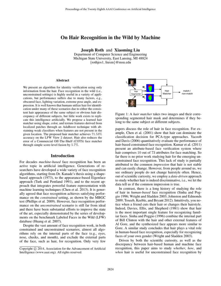
Figure 1: A hair matcher takes two images and their corresponding segmented hair mask and determines if they belong to the same subject or different subjects.
papers discuss the role of hair in face recognition. For example, Chen et al. (2001) show that hair can dominate the
classification decision for PCA-type approaches. Yacoob
and Davis (2006) quantitatively evaluate the performance of
hair-based constrained face recognition. Kumar et al. (2011)
present an attribute-based face verification system where
hair comprises 10 out of 73 attributes for face matching. So
far there is no prior work studying hair for the emerging unconstrained face recognition. This lack of study is partially
attributed to the common impression that hair is not stable
and can easily change. However, from people around us, we
see ordinary people do not change hairstyle often. Hence,
out of scientific curiosity, we employ a data-driven approach
to study whether hair is indeed discriminative, i.e., we let the
data tell us if the common impression is true.
In contrast, there is a long history of studying the role
of hair in human-based face recognition (Sinha and Poggio 1996; Wright and Sladden 2003; Johnston and Edmonds
2009; Toseeb, Keeble, and Bryant 2012). Intuitively, you notice when a friend cuts their hair or changes their hairstyle.
Indeed, Davies, Ellis, and Shepherd (1981) show that hair
is the most important single feature for recognizing familiar faces. Sinha and Poggio (1996) combine the internal part
of Bill Clinton with the hair and other external features of
Al Gore, and the synthesized face appears more similar to
Gore. A similar study concludes that hair plays a vital role
in human-based face recognition, especially for recognizing
faces of your own gender (Wright and Sladden 2003).
Driven by both the scientific curiosity, as well as the
discrepancy between hair-based human and machine face
recognition, this paper aims to study whether, how, and
when hair is useful for unconstrained face recognition by
Introduction
For decades machine-based face recognition has been an
active topic in artificial intelligence. Generations of researchers have developed a wide variety of face recognition
algorithms, starting from Dr. Kanade’s thesis using a shapebased approach (1973), to the appearance-based Eigenface
approach (Turk and Pentland 1991), and to the recent approach that integrates powerful feature representation with
machine learning techniques (Chen et al. 2013). It is generally agreed that face recognition achieves satisfying performance on the constrained setting, as shown by the MBGC
test (Phillips et al. 2009). However, face recognition performance on the unconstrained scenario is still far from ideal
and there have been substantial efforts to improve the state
of the art, especially demonstrated by the series of developments on the benchmark Labeled Faces in the Wild (LFW)
database (Huang et al. 2007).
Despite the vast amount of face recognition work, in both
constrained and unconstrained scenarios, almost all algorithms rely on the internal parts of the face (e.g., eyes,
nose, cheeks, and mouth), and exclude the external parts
of the face, such as hair, for recognition. Only very few
c 2014, Association for the Advancement of Artificial
Copyright Intelligence (www.aaai.org). All rights reserved.
2824
a machine. On the other hand, our study is also motivated
and enabled by a number of exciting recent research on
hair segmentation or labeling (Scheffler, Odobez, and Marconi 2011; Lee et al. 2008; Wang, Ai, and Tang 2012;
Kae et al. 2013; Wang et al. 2013), which substantially improve the segmentation accuracy on unconstrained facial images. For instance, the advanced hair labeling approach from
Kae et al. (2013) achieves 95% accuracy compared to the
ground truth at the superpixel level. The availability of excellent hair segmentation and the needs for improved face
recognition enable us to study this interesting topic.
Unlike conventional face recognition that uses only the internal parts of two faces, this paper studies how to perform
face recognition by using a complementary part, the hair regions, of two faces. We assume that a good quality hair segmentation has been conducted on two images. As shown in
Fig. 1, our central task is to design a discriminative feature
representation and classifier, termed “hair matcher”, to compute the similarity between two hair regions. Since hair is
a highly non-rigid object, we decide to use a local patchbased approach for feature representation. Given two faces
aligned by their eye locations, we have a series of rays emitting from the center of two eyes and intersecting with the
contour of the hair. We use the hair segmenter from Kae et
al. (2013) to identify the hair mask. The intersection points
will determine the local patches where we compute a rich set
of carefully designed hair features, including Bag of Words
(BoW)-based color features, texture features, and hair maskbased shape features. We use a boosting algorithm to select the features from local patches to form a classifier. Our
boosting algorithm can abstain at the weak classifier level
based on the fact that hair may not be present at some local
patches (Schapire and Singer 1999).
Our work differs from the prior work of Yacoob and
Davis (2006) and Kumar et al. (2011) in three aspects: 1)
we focus on unconstrained face recognition with greater hair
variations, 2) we employ a local patch driven approach to
optimally combine a wide variety of carefully designed features rather than using global descriptors from human intelligence such as split location, length, volume, curls, etc., 3)
we explicitly study the fusion of hair with face, which is critical for applying hair recognition to real-world applications.
In summary, this paper has a number of contributions:
We develop a hair matcher for unconstrained face recognition and evaluate on the standard LFW database. This is
the first known reported result from hair only on this de facto
database of unconstrained face recognition.
We demonstrate that hair and face recognition are uncorrelated and fail under different circumstances which allows for improvement through fusion.
We use basic fusion techniques with the proposed hair
matcher and a COTS face matcher and demonstrate improved face verification performance on the LFW database.
uq0i
i
uq2
Ii
Mi
i
uq0
j
uq2
c
θQ
θ0
Ij
Mj
Figure 2: Patch localization: Green region R40 is extracted
from the center of the ray independently for each image and
is used to compute color and texture features. Red region
R30 is extracted from only Ii and mapped to the same location in Ij and is used to compute shape features.
a function, F (Ii (Mi ), Ij (Mj )), that returns a large value if
the images belong to the same subject, or otherwise a small
value. This paper assumes that the hair mask Mi can be obtained automatically through a hair segmenter.
Alignment is often the first step for any object recognition
system (Liu et al. 2008; Liu 2009), such that the topologically equivalent parts are compared with each other. Unlike
rigid objects where alignment is easy w.r.t. a standard object
instance, hair is a highly non-rigid object where the alignment between two hair regions does not appear straightforward. Fortunately, hair attaches to the head, which is relatively more rigid compared to hair and can be better aligned
via the face. Therefore, given an image pair, we first align
their face regions, and the aligned images are the input (Ii
and Ij ) to the proposed algorithm. Specifically, in the LFW
database, we choose to work on the funneled dataset (Huang,
Jain, and Learned-Miller 2007) where all face regions are
reasonably aligned with the in-plane rotation (roll) removed.
Patch localization: Similar to any object recognition system, the hair matcher requires an effective feature representation. We choose to use a local feature-based representation
due to two considerations. 1) Hair may have distinct local
properties (e.g., texture, shape, color) across one part of the
hair region. 2) Local representation is potentially more robust to the hair segmentation error, which is typically nonuniformly distributed over the hair region.
In order to consistently localize patches for feature extraction, we propose a ray-based sampling method. As shown
in Fig. 2, given the center (c) of two average eye locations
in the dataset, we define a line function lq (u; θq ) = 0 that
passes through c with a horizontal angle θq . (We cannot use
an image-specific eye center without violating the restricted
protocol of LFW). By varying θq within a range, specifically
q 5π
π
θq = Q
3 − 3 for q ∈ [0, Q] and Q = 106, a collection of
line functions are generated. This range ignores the locations
beneath the face where very few images have hair. We denote the set of boundary pixels of a hair mask M as B, which
describes the internal and external hair lines. It is expected
that in many cases the line function will intersect with B,
and the collection of intersected points of all lines is denoted
as {uq , u0 q }, where lq (uq ) = lq (u0 q ) = 0, {uq , u0 q } ∈ B.
We sample patches at five equidistant locations along each
0
line lq at uqp = p4 uq + 4−p
4 u q for p ∈ [0, 4]. From now on
Hair Recognition Approach
Hair Matcher Framework
Given a pair of images Ii and Ij , along with their corresponding hair masks Mi and Mj , a hair matcher consists of
2825
{uqp } defines the local patch centers for extracting various
feature representations. Note that depending on the shape
of hair, {uqp } may contain empty elements for a subset of
θq . This implies that no local feature will be extracted from
these patch locations, and we will handle this missing feature issue by our classifier learning algorithm.
bits change values more than twice are mapped to the same
pattern, leaving only 59 unique patterns. This mapping is
denoted as LBP8,2 . A histogram of the patterns within the
h
l
patch is used as the LBP feature, i.e., fqr
= ||h||
, where
1
P
h(j) = (u,v)∈Rr δ(LBP8,2 (u, v) = j)δ(M(u, v) = 1).
For HOG-like features, we compute the histogram using
nine orientations evenly spaced between 0 and π. The feah
ture fqr
is the normalized histogram of the sum of all gradients with the given orientation. Our system differs from
Dalal’s HOG in that we use the whole region Rr as a single
cell instead of sampling multiple cells within a block. This
g
l
h
leaves us with a 6Q-dim texture feature f t = {fqr
, fqr
, fqr
}
per image.
Feature Extraction
Hair Color Features The Fischer-Saller scale is used in
physical anthropology and medicine to describe the hair
color distribution, where a series of scales is defined from
light blond to red blond (Hrdy 1978). Inspired by this,
we use a data driven approach to learn the distribution (or
codes) of hair color in our training dataset. Specifically,
we convert all hair pixels within the N training images,
{Ii (Mi )}i∈[1,N ] , from the RGB space to the HSV space. In
order to learn the representative hair color, one would typically perform a K-means clustering in the 3-dim HSV space.
However, Euclidean distances perform poorly for clustering
the polar coordinates of HSV. Specifically, when the value
(V) is small, colors are very similar regardless of the hue
(H) or saturation (S). To remedy these issues, we scale S by
V to create a conical space, and then perform K-means clustering on its Cartesian representation. As shown in Fig. 3,
the resultant dc = 20 color codes, [s1 , s2 , · · · , sdc ], appear
to cover a wide range of typical hair colors.
Given one image I, we use the center point along each line
uq2 . For each hair pixel within an r × r patch Rr around uq2
where r ∈ {21, 41}, we search for its nearest color code.
c
=
For each patch, we generate a dc -dim BoW histogram fqr
h
||h||1 , where
h(d) =
P
(u,v)∈Rr
Hair Shape Features Hair shape can be described solely
by the internal and external hair lines. Ideally for the genuine match, both hair lines of one image should overlap with
those of the other image. However, due to the potential discrepancy in head poses, such overlap may not happen everywhere along the hair lines. To remedy this issue, one approach is to perform a 3D hair model fitting on one image,
rotate the head to the same pose as the other image, and synthesize the hair lines under the new pose. Considering the
challenger of 3D hair fitting for unconstrained images, we
take an alternative approach to search for the local regions
that have more consistent hair lines under pose variations.
Unlike the color and texture, where only the center between two hair boundary points is used for feature extraction, for the shape feature we use all five uqp points along
each line. For each point, we use the hair mask within its los
cal patch as the shape feature, fqpr
= M(u), ∀u ∈ Rr (uqp ),
where the patch size r = {11, 21, 31}.
For the color and texture, the two matching images, Ii and
Ij , have different patch locations for feature extraction, uiq2
and ujq2 . In contrast, for shape, both images extract features
from the same locations, which are uqp of one of the two
j
i
=
= Mi (u), ∀u ∈ Rr (uiqp ) and fqpr
images. That is, fqpr
i
Mj (u), ∀u ∈ Rr (uqp ) are the local shape features of Ii and
Ij . The shape feature for an image pair is defined as,
j
i
(u) = fqpr
(u) = 1,
if fqpr
1,
s
i
j
(1)
xqpr (u) = 0,
if fqpr (u) = fqpr (u) = 0,
−1, otherwise,
δ(d = arg mind ||I(u, v) − sd ||2 )δ(M(u, v) = 1),
and δ() is the indicator function. The collection of all patchbased color histograms constitutes the color feature for the
c
}.
image I, f c = {fqr
Hair Texture Features Many texture features are used in
vision applications and we use Gabor filter (Liu and Chaudhuri 2002), Local Binary Patterns (LBP) (Ojala, Pietikainen,
and Maenpaa 2002), and an oriented gradient feature similar to Histogram of Oriented Gradients (HOG) (Dalal and
Triggs 2005). Gabor filter has been widely used in face
recognition as a low-level feature representation. We choose
it to describe hair texture due to its capability in capturing
hair orientation. Specifically, the Gabor filter is defined as:
Gx,y (λ, θ, ψ, σ, γ) =
0
02
2 02
0
y
exp(− x +γ
) exp(i(2π xλ
2σ 2
0
where xsqpr is a r2 -dim vector. This definition allows us to
treat differently the pixels being both hair or both background. Note that it is important to ensure that the feature
comparison is conducted only for the pixels at the same location, otherwise the hairs with different thickness would
also match well based on the shape feature definition.
Given an image pair Ii and Ij , we represent the visual
similarity of two hair regions via the joint feature vector,
x = [xc , xt , xs ] = [|fic − fjc |, |fit − fjt |, {xsqpr }]. There are
2Q color features with the dimension of dc , 6Q texture features with the dimension of 40, 59, or 9, and 15Q shape features with the dimension of r2 . Depending on whether two
images are of the same subject, x will be used as a positive
or negative training sample for learning a hair matcher.
+ ψ)),
where x = x cos(θ) + y sin(θ), y = −x sin(θ) + y cos(θ).
By setting ψ = π2 , σ = 2, γ = 0.5, λ = {0.5, 1, · · · , 2.5},
and θ = { π8 , 2π
8 , · · · , π}, we have 40 different Gabor filters and their convolution with an image I generates 40 filter responses GIj = I ∗ G(λ, θ). Similar to the color feature, for each patch Rr (uq2 ), we compute the texture feag
ture, which is a 40-dim vector fqr
with each element being the mean of
the
real
part
of
the filter responses, i.e.,
P
1
g
I
fqr
(j) = ||u||
(u,v)∈Rr Re(Gj (u, v))δ(M(u, v) = 1).
1
LBP creates an 8-bit number for each u by thresholding
the 8-neighborhood by I(u). All numbers where consecutive
2826
Algorithm 1: Learning a hair matcher via boosting.
Data: Samples and labels {xn , yn }n∈[1,N ] , with
yn ∈ {−1, +1}.
Result: The hair matcher classifier F .
Initialize the weights wn = N1 , and F = 0.
foreach m = 1, · · · , M1 do
foreach v = 1, · · · , 23Q do
PN
v
v
2
arg min
n=1 1(xn )wn (f (xn ; w, τ, p) − yn ) ,
Figure 3: Example DML matrix A. Note colors from specular reflection (e.g., Code 1 and 3) have little impact on the
similarity s as all values are close to zero.
w,τ,p
where 1(xvn ) = 0 if xvn is abstained and 1 otherwise,
and
if pw| xvn > τ,
1,
v
f (xn ; w, τ, p) = −1, if pw| xvn < τ,
(2)
0,
if f abstains on xvn .
P
(f (xvn ) = yn ),
Wc = N1
Pn
1
Wm = N n (f (xvn ) 6= yn ),
P
v
Wa = N1
n (f (xn ) = 0).
√
Select fm with minimal Z = Wa + 2 Wc Wm . Quit if
Z = 1.
If fm uses a color feature, compute A via DML.
Wc
Compute αm = 12 log( W
) and update the weights:
m
w
n
q
, if fm misclassifies xn ,
W
+2Wm
Wa Wm
c
w
q n
wn =
(3)
, if fm classifies xn ,
Wc
W
+2Wc
wna Wm
,
if fm abstains on xn .
Z
P
Normalize the weights wn such that n wn = 1.
PM1
return F (x) = m=1 αm fm (x; w, τ, p).
Specifically, a full rank matrix A, rather than a vector, is
learned to project the features as follows:
s = p(fi − fj )| A(fi − fj ),
(5)
according to the objective function:
X
min
||fi − fj ||2A
A
s.t.
(fi ,fj )∈N +
X
||fi − fj ||2A ≥ 1, A 0,
(6)
(fi ,fj )∈N −
where N + and N − are the genuine and impostor training
samples respectively. Figure 3 shows one resultant A matrix.
Boosting with Abstaining Features One unique aspect of
our problem is that for any local feature, it is possible that
one image or both images of a certain pair do not have feature values, because no hair is present in that specific local
patch. Therefore, we decide to use boosting with abstaining features for our problem (Schapire and Singer 1999;
Smeraldi, Defoin-Platel, and Saqi 2010), which can specifically consider absent features during feature selection.
Algorithm 1 presents the key steps in our boosting-based
learning. We learn a similarity measure for each individual
feature in order to use the conventional stump classifier with
a threshold τ and a parity p. Unlike conventional boosting,
the sample with an absent feature has a classifier output of
0 (Eq. 2) and does not participate in the estimation of stump
classifier parameters (w, τ , p). The weak classifier is selected not only by the amount of samples that are classified
correctly (Wc ) and misclassified (Wm ), but also by those
that have abstained features (Wa ). This prevents the feature
selection from favoring a feature where many samples have
abstained. Similarly, these three values also determine the
updating of the sample weights. Note that for efficiency we
do not compute DML for every color-based stump classifier
during the iteration, but rather wait until the iteration has
completed. Finally, the boosting procedure results in a hair
matcher, which is a weighted summation of M1 weak classifiers each with associated parameters (w or A, τ , p).
Classifier Learning
Similarity Measurement Having extracted the feature
representation for both genuine matches and impostor
matches, now we need to learn a classifier to separate these
two classes. Given the high dimensionality of the feature
space, we choose to use boosting due to its known advantage
in combining both feature selection and classifier learning in
one step, as well as its success in many vision problems (Viola and Jones 2004). A major part of any boosting framework is to learn weak stump classifiers. We choose to learn
a simple similarity measure for a given local feature vector
by projecting xn = |fi − fj | to a scalar, and then performing classification by a simple threshold τ . Similar to Liu and
Yu (2007), this projection can be done efficiently through
Linear Discriminant Analysis (LDA) to learn a vector w to
maximize the difference between two classes. Since higher
similarity values for the genuine match is desired, a parity p
is used to flip the sign after the projection:
s = pw| xn .
(4)
Learning the LDA projection is computationally efficient,
but it fails to consider the correlation between different dimensions of the local feature vector. For the texture and
shape features, there is minimal correlation, but for the color
features there is correlation between similar color codes especially since lighting can impact the color. Distance Metric Learning (DML) (Xing et al. 2003) is designed to learn
a projection that considers the correlation among features.
Fusion with COTS Face Matcher
Since hair is not dependent on face occlusion or expression, we aim to create a fusion scheme where a COTS face
matcher can benefit from the proposed hair matcher. We plan
to fuse at the score level since that is the highest level possible with a black box COTS system.
2827
(a)
(b)
(c)
Figure 5: Examples of hair matcher performance. Correct samples with the greatest |F (x)| (a), random correct samples (b), and
incorrect samples with the greatest |F (x)| (c).
1
0.8
TPR
0.6
Eigenfaces
Fisher
Texture
Shape
Color
Combined
0.4
0.2
0
0
0.2
0.4
0.6
0.8
(a)
(b)
(c)
Figure 6: Distribution of shape (red), texture (green), and
color (blue) features chosen by boosting. First 20 (a), top 20
by weights α (b), and all 200 (c) features.
1
FPR
Figure 4: ROC comparison of Eigenfaces, Hair, and Fisher
vector faces on LFW View 2.
et al. 2007). LFW is popular due to its unconstrained nature, difficulty, well-defined protocol, and the availability
of results of prior work. To ensure hair alignment between
two images, the funneled version of LFW is used (Huang,
Jain, and Learned-Miller 2007). We use the hair segmenter
from Kae et al. (2013). The database consists of 13, 233,
250x250 pixel images from 5, 749 individuals. We follow the restricted View 2 protocol, where 3, 000 genuine
matches and 3, 000 impostor matches are divided into 10
equal size partitions for cross validation.
We employ the standard Receiver Operating Characteristic (ROC) curve for performance evaluation. The ROC curve
is defined on two axes: False Positive Rate (FPR), the fraction of impostor matches incorrectly accepted to be genuine, and True Positive Rate (TPR), the fraction of genuine
matches correctly classified as genuine. To summarize the
ROC curve, we use the Equal Error Rate (EER), which is
when FPR equals 1−TPR, and the accuracy (1−EER).
Figure 4 displays the performance of the proposed hair
matcher with the original Eigenfaces (Turk and Pentland
1991) and the state-of-the-art Fisher vector faces (Simonyan
et al. 2013). We run the hair matcher using shape, color, and
texture features independently in order to demonstrate their
individual effectiveness. They perform nearly the same, and
when combined, the learned hair matcher achieves 71.53%
accuracy. As no other hair technique is designed for the unconstrained setting nor tested on LFW, this is the first reported result using a hair matcher on LFW. Figure 5 displays
samples where the hair matcher succeeds and fails.
Selected Features: Figure 6 shows the features selected by
boosting. This specific matcher selects 123 shape features,
69 texture features, and 8 color features. Even though color
performs well by itself, it has fewer overall selections. We
hypothesize that this is due to DML only being computed if
The first step to fusion is to choose a suitable scorenormalization. We desire a technique that reduces the effect of outliers and is also unaffected by the non-Gaussian
impostor distribution of the COTS matcher. To fulfill these
needs, we choose to use the tanh normalization (Jain, Nandakumar, and Ross 2005), which is based on the mean µ and
standard deviation σ of the genuine training samples using:
F (x) − µ
1
0
) +1 .
(7)
tanh 0.01(
F (x) =
2
σ
The second step is to combine the normalized scores,
where standard techniques include min, max, and mean.
Since we have enough training data, we use a Support Vector
Machine (SVM) with a standard radial basis kernel to form
a final classification decision instead.
There are certain instances where either hair or face can
produce poor results, e.g., obscurity through a hat or sunglasses. In the future, we can further improve the fusion
performance by estimating quality metrics for both face and
hair and feed them to the SVM. This will make a decision
based not only on the raw score, but also on which metric
will work best for the given conditions.
Experimental Results
In this section, we evaluate the proposed hair matcher in the
unconstrained face recognition scenario. We seek to understand when the hair matcher succeeds and under what scenarios it can improve face recognition.
Hair Matcher
To evaluate the proposed algorithm, we use the de facto
database for unconstrained face recognition, LFW (Huang
2828
Figure 9: Sweetspot pairs: Samples where fusion successfully corrects misclassified pairs by the COTS system.
G
21
7.83%
Hair (Fh )
Hair (Fh )
21
−0.056
I
4.8%
Table 1: Accuracy comparison
4.17%
G
Matcher
Full resolution
Quarter resolution
−0.056
−10.7
−1.5 I−1.33 G 15
COTS (Ff )
8.43%
I
−10.7
−1.5 I−1.33 G 15
COTS (Ff )
(a)
(b)
1
0.8
TPR
0.6
Hair
COTS
Fusion
Hair4
COTS4
Fusion4
0.2
0
0
0.2
0.4
0.6
0.8
COTS
87.38%
79.69%
Fused
88.10%
82.37%
ROC curve in Fig. 8. This fusion scheme increases the COTS
performance from 87.38% to 88.10%, which is a 5.7% reduction of the error. Although minor in improvement, the
paired t-test has a statistically significant p-value of 0.014.
This demonstrates that hair is able to improve the face recognition performance. In the future, we will develop face and
hair quality metrics to better predict sweetspot pairs.
Figure 9 demonstrates examples where the fused matcher
corrects errors made by the COTS. We make the following
remarks from these examples. Face recognition can be significantly hindered by obstructions (e.g., sunglasses), poor
focus, expression, lighting, and pose variation. Hair works
without respect to expression or obstructions, and the degradation due to pose, focus, and lighting is less than face.
Low Resolution: To examine the degradation of the proposed hair matcher w.r.t. image resolution, we downsample
the LFW database to 63 × 63 pixel images (quarter resolution). Since we are interested only in the performance of
the hair matcher and not hair segmentation, we also downsample the hair masks directly. The reported results will be
achievable if/when hair segmentation works at the low resolution. At this resolution, the COTS matcher fails to enroll
(FTE) and produces no score for 14.8% of the pairs. To report the performance of COTS, we flip a coin when this occurs and assign the pair a random score from either the genuine or impostor distribution. When COTS produces a score,
the accuracy is 84.86%, but the FTE cases cause the accuracy to drop to 79.69%. Hair recognition degrades gracefully
at the reduced resolution, so we modify the fusion scheme
to use only Fh whenever FTE occurs. Fusion appears to be
more effective and has an error reduction of 13.20%. The
exact performance results are presented in Tab. 1 and Fig. 8.
Figure 7: Distributions of COTS and hair scores for genuine
(a) and impostor samples (b). G and I on the axes refer to
matcher’s classification decision as genuine or imposter.
0.4
Hair
71.53%
68.63%
1
FPR
Figure 8: ROC comparison of COTS, hair matcher, and
fused results on full and quarter resolution images.
a color feature is chosen through the weaker LDA. Despite
this disadvantage, color is still important, since a color feature near the top of the head is almost always chosen first
with a high weight. Because the boosting algorithm may abstain, it is possible to have higher weighted features appearing at later iterations. As seen in the middle image, these top
weighted features tend to be beneath the ears where fewer
images have hair, but when present is highly discriminative.
Fusion with COTS Face Matcher
The proposed hair matcher performs well, but it is still behind the state-of-the-art performance of face recognition. We
seek to determine the usefulness of the hair matcher by fusing with PittPatt V5.2 (pit 2011), one of the best performing
COTS face matchers. Figure 7 shows the joint distribution of
Ff and Fh .The Pearson correlation coefficient is 0.4, which
indicates low correlation, and thus fusion has the potential
to improve performance. Each axis is scaled piecewise linearly to provide equal space for the genuine and impostor
decisions and the overlay shows the percentage of samples
occurring in the cases where COTS fails. We call the regions
where hair succeeds but face fails the sweetspot and 8.13%
of testing image pairs fall into these regions. If there exists a
perfect fusion scheme, hair would improve the performance
of the COTS to 95.5%, which indicates the great promise of
fusing hair with face recognition.
Using SVM on tanh normalized scores, we generate the
Conclusions
With a structured and data-driven approach, we presented
the first work for automated face recognition using only hair
features in the unconstrained setting. On the de facto LFW
dataset, we showed the usefulness of our fully automatic hair
matcher by itself and by improving a COTS face matcher.
Through the answers of whether, how and when hair is useful for unconstrained face recognition, this work made a notable contribution to this important problem, and warranted
further study on hair, the often-ignored visual cue.
Acknowledgement
We thank Andrew Kae and Erik Learned-Miller in kindly
providing the hair segmentation masks of the LFW images.
2829
References
Ojala, T.; Pietikainen, M.; and Maenpaa, T. 2002. Multiresolution gray-scale and rotation invariant texture classification
with local binary patterns. IEEE Trans. Pattern Anal. Mach.
Intell. 24(7):971–987.
Phillips, P. J.; Flynn, P. J.; Beveridge, J. R.; Scruggs, W. T.;
O’Toole, A. J.; Bolme, D.; Bowyer, K. W.; Draper, B. A.;
Givens, G. H.; Lui, Y. M.; Sahibzada, H.; Scallan, Iii, J. A.;
and Weimer, S. 2009. Overview of the multiple biometrics
grand challenge. In Proc. Int. Conf. Biometrics (ICB), 705–
714.
2011. PittPatt Software Developer Kit, http://www.pittpatt.
com.
Schapire, R., and Singer, Y. 1999. Improved boosting algorithms using confidence-rated predictions. Mach. Learning
37(3):297–336.
Scheffler, C.; Odobez, J.-M.; and Marconi, R. 2011. Joint
adaptive colour modelling and skin, hair and clothing segmentation using coherent probabilistic index maps. In Proc.
British Machine Vision Conf. (BMVC), 53.1–53.11.
Simonyan, K.; Parkhi, O. M.; Vedaldi, A.; and Zisserman,
A. 2013. Fisher vector faces in the wild. In Proc. British
Machine Vision Conf. (BMVC), 8.1–8.12.
Sinha, P., and Poggio, T. 1996. I think i know that face...
Nature 384:404.
Smeraldi, F.; Defoin-Platel, M.; and Saqi, M. 2010. Handling missing features with boosting algorithms for proteinprotein interaction prediction. In Data Integration in the Life
Sciences, 132–147. Springer.
Toseeb, U.; Keeble, D. R.; and Bryant, E. J. 2012. The significance of hair for face recognition. PLoS ONE 7(3):e34144.
Turk, M., and Pentland, A. 1991. Eigenfaces for recognition.
Journal of Cognitive Neuroscience 3(1):71–86.
Viola, P., and Jones, M. 2004. Robust real-time face detection. Int. J. Comput. Vision 57(2):137–154.
Wang, N.; Ai, H.; and Tang, F. 2012. What are good parts for
hair shape modeling? In Proc. IEEE Conf. Computer Vision
and Pattern Recognition (CVPR), 662–669.
Wang, D.; Shan, S.; Zhang, H.; Zeng, W.; and Chen, X.
2013. Isomorphic manifold inference for hair segmentation.
In Proc. Int. Conf. Automatic Face and Gesture Recognition
(FG), 1–6.
Wright, D. B., and Sladden, B. 2003. An own gender bias and
the importance of hair in face recognition. Acta Psychologica
114(1):101 – 114.
Xing, E. P.; Ng, A. Y.; Jordan, M. I.; and Russell, S. 2003.
Distance metric learning, with application to clustering with
side-information. In Advances in Neural Information Processing Systems (NIPS), 505–512.
Yacoob, Y., and Davis, L. 2006. Detection and analysis of
hair. IEEE Trans. Pattern Anal. Mach. Intell. 28(7):1164–
1169.
Chen, L.-F.; Liao, H.-Y. M.; Lin, J.-C.; and Han, C.-C. 2001.
Why recognition in a statistics-based face recognition system should be based on the pure face portion: a probabilistic decision-based proof. Pattern Recognition 34(7):1393 –
1403.
Chen, D.; Cao, X.; Wen, F.; and Sun, J. 2013. Blessing
of dimensionality: High-dimensional feature and its efficient.
compression for face verification. In Proc. IEEE Conf. Computer Vision and Pattern Recognition (CVPR), 3025–3032.
Dalal, N., and Triggs, W. 2005. Histograms of oriented gradients for human detection. In Proc. IEEE Conf. Computer
Vision and Pattern Recognition (CVPR), volume 1, 886–893.
Davies, G.; Ellis, H.; and Shepherd, J. 1981. Perceiving and
Remembering Faces. New York: Academic Press.
Hrdy, D. 1978. Analysis of hair samples of mummies from
semna south. American J. of Physical Anthropology 49:277–
282.
Huang, G. B.; Ramesh, M.; Berg, T.; and Learned-Miller, E.
2007. Labeled faces in the wild: A database for studying
face recognition in unconstrained environments. Technical
Report 07-49, University of Massachusetts, Amherst.
Huang, G. B.; Jain, V.; and Learned-Miller, E. 2007. Unsupervised joint alignment of complex images. In Proc. Int.
Conf. Computer Vision (ICCV), 1–8.
Jain, A. K.; Nandakumar, K.; and Ross, A. 2005. Score normalization in multimodal biometric systems. Pattern Recognition 38(12):2270–2285.
Johnston, R. A., and Edmonds, A. J. 2009. Familiar and
unfamiliar face recognition: A review. Memory 17(5):577–
596.
Kae, A.; Sohn, K.; Lee, H.; and Learned-Miller, E. 2013.
Augmenting CRFs with Boltzmann machine shape priors for
image labeling. In Proc. IEEE Conf. Computer Vision and
Pattern Recognition (CVPR), 2019–2026.
Kanade, T. 1973. Picture Processing System by Computer
Complex and Recognition of Human Faces. Ph.D. Dissertation, Kyoto University, Kyoto, Japan.
Kumar, N.; Berg, A.; Belhumeur, P. N.; and Nayar, S.
2011. Describable visual attributes for face verification
and image search. IEEE Trans. Pattern Anal. Mach. Intell.
33(10):1962–1977.
Lee, K.-C.; Anguelov, D.; Sumengen, B.; and Gokturk, S.
2008. Markov random field models for hair and face segmentation. In Proc. Int. Conf. Automatic Face and Gesture
Recognition (FG), 1–6.
Liu, C., and Chaudhuri, A. 2002. Reassessing the 3/4 view
effect in face recognition. Cognition 83(1):31–48.
Liu, X., and Yu, T. 2007. Gradient feature selection for online
boosting. In Proc. Int. Conf. Computer Vision (ICCV), 1–8.
Liu, X.; Yu, T.; Sebastian, T.; and Tu, P. 2008. Boosted
deformable model for human body alignment. In Proc. IEEE
Conf. Computer Vision and Pattern Recognition (CVPR), 1–
8.
Liu, X. 2009. Discriminative face alignment. IEEE Trans.
Pattern Anal. Mach. Intell. 31(11):1941–1954.
2830
