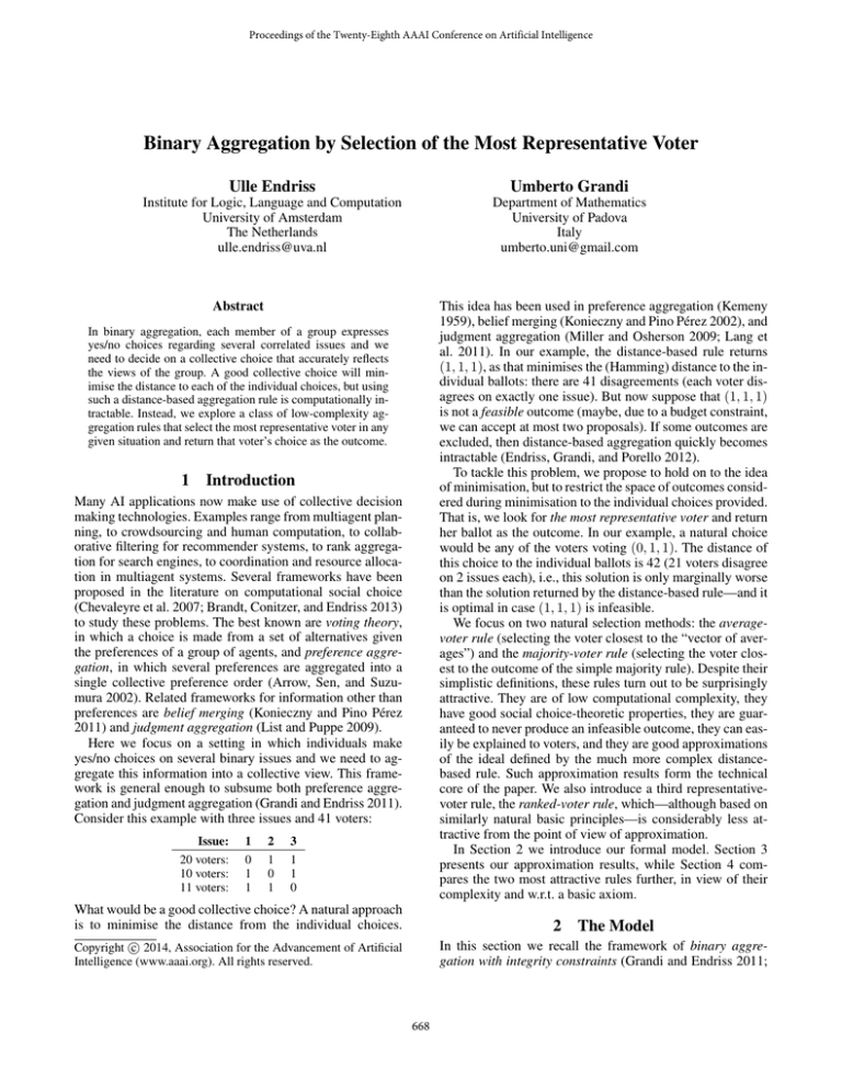
Proceedings of the Twenty-Eighth AAAI Conference on Artificial Intelligence
Binary Aggregation by Selection of the Most Representative Voter
Ulle Endriss
Umberto Grandi
Institute for Logic, Language and Computation
University of Amsterdam
The Netherlands
ulle.endriss@uva.nl
Department of Mathematics
University of Padova
Italy
umberto.uni@gmail.com
Abstract
This idea has been used in preference aggregation (Kemeny
1959), belief merging (Konieczny and Pino Pérez 2002), and
judgment aggregation (Miller and Osherson 2009; Lang et
al. 2011). In our example, the distance-based rule returns
(1, 1, 1), as that minimises the (Hamming) distance to the individual ballots: there are 41 disagreements (each voter disagrees on exactly one issue). But now suppose that (1, 1, 1)
is not a feasible outcome (maybe, due to a budget constraint,
we can accept at most two proposals). If some outcomes are
excluded, then distance-based aggregation quickly becomes
intractable (Endriss, Grandi, and Porello 2012).
To tackle this problem, we propose to hold on to the idea
of minimisation, but to restrict the space of outcomes considered during minimisation to the individual choices provided.
That is, we look for the most representative voter and return
her ballot as the outcome. In our example, a natural choice
would be any of the voters voting (0, 1, 1). The distance of
this choice to the individual ballots is 42 (21 voters disagree
on 2 issues each), i.e., this solution is only marginally worse
than the solution returned by the distance-based rule—and it
is optimal in case (1, 1, 1) is infeasible.
We focus on two natural selection methods: the averagevoter rule (selecting the voter closest to the “vector of averages”) and the majority-voter rule (selecting the voter closest to the outcome of the simple majority rule). Despite their
simplistic definitions, these rules turn out to be surprisingly
attractive. They are of low computational complexity, they
have good social choice-theoretic properties, they are guaranteed to never produce an infeasible outcome, they can easily be explained to voters, and they are good approximations
of the ideal defined by the much more complex distancebased rule. Such approximation results form the technical
core of the paper. We also introduce a third representativevoter rule, the ranked-voter rule, which—although based on
similarly natural basic principles—is considerably less attractive from the point of view of approximation.
In Section 2 we introduce our formal model. Section 3
presents our approximation results, while Section 4 compares the two most attractive rules further, in view of their
complexity and w.r.t. a basic axiom.
In binary aggregation, each member of a group expresses
yes/no choices regarding several correlated issues and we
need to decide on a collective choice that accurately reflects
the views of the group. A good collective choice will minimise the distance to each of the individual choices, but using
such a distance-based aggregation rule is computationally intractable. Instead, we explore a class of low-complexity aggregation rules that select the most representative voter in any
given situation and return that voter’s choice as the outcome.
1
Introduction
Many AI applications now make use of collective decision
making technologies. Examples range from multiagent planning, to crowdsourcing and human computation, to collaborative filtering for recommender systems, to rank aggregation for search engines, to coordination and resource allocation in multiagent systems. Several frameworks have been
proposed in the literature on computational social choice
(Chevaleyre et al. 2007; Brandt, Conitzer, and Endriss 2013)
to study these problems. The best known are voting theory,
in which a choice is made from a set of alternatives given
the preferences of a group of agents, and preference aggregation, in which several preferences are aggregated into a
single collective preference order (Arrow, Sen, and Suzumura 2002). Related frameworks for information other than
preferences are belief merging (Konieczny and Pino Pérez
2011) and judgment aggregation (List and Puppe 2009).
Here we focus on a setting in which individuals make
yes/no choices on several binary issues and we need to aggregate this information into a collective view. This framework is general enough to subsume both preference aggregation and judgment aggregation (Grandi and Endriss 2011).
Consider this example with three issues and 41 voters:
Issue:
1
2
3
20 voters:
10 voters:
11 voters:
0
1
1
1
0
1
1
1
0
What would be a good collective choice? A natural approach
is to minimise the distance from the individual choices.
2
The Model
In this section we recall the framework of binary aggregation with integrity constraints (Grandi and Endriss 2011;
c 2014, Association for the Advancement of Artificial
Copyright Intelligence (www.aaai.org). All rights reserved.
668
2013). It is a variant of both binary aggregation with explicitly specified feasible sets (Dokow and Holzman 2010) and
judgment aggregation (List and Puppe 2009), and all of our
results can easily be translated into these other frameworks
as well. We also define several concrete aggregation rules.
2.1
An aggregation rule is called collectively rational w.r.t. an
integrity constraint IC if all elements of F (B) satisfy IC
whenever B is rational, i.e., whenever all Bi satisfy IC.
2.2
The Hamming distance between ballot B = (b1 , . . . , bm )
and ballot B 0 = (b01 , . . . , b0m ) is defined as the number of
issues on which they differ:
H(B, B 0 ) = |{j ∈ I | bj 6= b0j }|
Basic Definitions
Let I = {1, . . . , m} be a finite set of issues. We want
to model decision making problems where a group of voters have to jointly decide for which issues to choose “yes”
and for which to choose “no”. A ballot B is an element of
{0, 1}m , which associates each issue with either a 1 (“yes”)
or a 0 (“no”). We write bj for the jth element of ballot B.
Not every element of {0, 1}m might be a feasible or rational choice. For instance, if the issues are funding decisions,
then a budget constraint might mean that no outcome with
more than, say, five 1’s is feasible. We shall assume that the
same constraints apply to both individual ballots and outcomes. Let PS = {p1 , . . . , pm } be a set of propositional
variables, one for each issue in I. An integrity constraint is
a consistent formula IC in the language obtained from PS by
closing under the standard propositional connectives (¬, ∧,
∨, →, ↔). Let Mod(IC) ⊆ {0, 1}m be the set of models of
IC, i.e., the set of rational ballots satisfying IC.
Let N = {1, . . . , n} be a finite set of voters (with n > 2).
A profile is a vector of rational ballots B = (B1 , . . . , Bn ) ∈
Mod(IC)n , one for each voter. We write bi,j for the jth element of ballot Bi , the ith element of profile B. We write
B
Nj:x
= {i ∈ N | bi,j = x} for the set of voters choosing
value x ∈ {0, 1} for issue j in profile B. The support of a
profile B = (B1 , . . . , Bn ) is the set of all ballots that occur at least once within B: S UPP(B) = {B1 , . . . , Bn }. An
m
(irresolute) aggregation rule F : {0, 1}m×n → 2{0,1} is a
function that maps every profile B to a non-empty subset of
{0, 1}m . That is, F returns a set of ballots.
An example of a rule is the majority rule, which accepts
an issue if a majority of the voters do. In fact, there are two
possible definitions of “majority”: we may accept an issue
if at least half of the voters do (weak majority) or only if
more than half of them do (strict majority). We define Maj as
the irresolute aggregation rule that returns the set including
both the weak and the strict majority winner (which may or
may not coincide): Maj(B) = {B w , B s } with bw
j = 1 iff
n
n+1
B
s
B
|Nj:1 | > d 2 e and bj = 1 iff |Nj:1 | > d 2 e.
In the presence of an integrity constraint, a rule may
sometimes output an irrational ballot given a rational profile.
An example is the following scenario, in which the integrity
constraint IC = pC ↔ pA ∧ pB forces voters to accept issue
C if and only if the first two issues are accepted:1
Issue:
A
B
C
Voter 1:
Voter 2:
Voter 3:
0
1
1
1
0
1
0
0
1
Maj:
1
1
0
The Distance-Based Rule
For example, H((1, 0, 0), (1, 1, 1)) = 2. The Hamming distance between a ballot B and a profile B is the sum of the
Hamming distances between B and the ballots in B:
X
H(B, B) =
H(B, Bi )
i∈N
For S ⊆ {0, 1}m , by a slight abuse of notation, we will write
H(S, B) as a shorthand for {H(B, B)) | B ∈ S}.
Definition 1. Given an integrity constraint IC, the distancebased rule DBRIC is the following function:
DBRIC (B)
=
argmin H(B, B)
B∈Mod(IC)
Thus, winning ballots under the DBRIC are rational ballots
that minimise disagreement with the individual ballots. Note
that the DBRIC is collectively rational by definition (outcomes are chosen from Mod(IC)). Also note that the definition of the distance-based rule is dependent on the IC.
Fact 1. If IC = >, then DBRIC = Maj.
That is, if the IC does not restrict the set of ballots, the outcome of the DBR coincides with that of the majority rule.
Preference aggregation can be viewed as an instance of binary aggregation by devising a suitable integrity constraint:
issues are propositions of the form pab , and IC encodes the
properties of linear orders (Grandi and Endriss 2011). The
preference aggregation version of the DBRIC is known as
the Kemeny rule (1959), and is one of the most studied aggregation rules. However, it has a prohibitively high computational complexity: winner determination is Θp2 -complete
(Hemaspaandra, Spakowski, and Vogel 2005).
2.3
Rules Based on Representative Voters
A simple idea to reconcile distance minimisation with algorithmic efficiency is to restrict the search for a representative
collective view to the set of ballots submitted by the individuals. This gives rise to a class of aggregation rules known as
generalised dictatorships (Grandi and Endriss 2013). Rules
in this class are collectively rational for every possible IC,
and no rule outside this class has this desirable property.
Still, not all such rules are “good” rules: a proper dictatorship Fi : B 7→ Bi that chooses as collective outcome the
ballot of the same voter i in all profiles is certainly not attractive. The problem of selecting the most representative voter
is thus crucial to obtaining interesting rules in this class.
How should we select this “most representative voter” for
a given profile? There are several natural choices. Here we
define three of them, each inspired by an existing rule:
1
In the literature on judgment aggregation, this example is
known as the discursive dilemma (List and Puppe 2009).
669
Definition 5. Let F and F 0 be aggregation rules. Then F
is said to be an α-approximation of F 0 if H(F (B), B) 6
α · H(F 0 (B), B) for every profile B.
Recall that F (B) and F 0 (B) are sets of outcomes. Above
inequality is understood to apply to all elements of these
sets, i.e., max[H(F (B), B)] 6 α · min[H(F 0 (B), B)].
Thus, the worst F -winner has a distance to the profile that
is at most α times the distance from the best F 0 -winner to
the profile. F is called a strict α-approximation of F 0 , if the
inequality is strict (when the second distance is not zero).
As a first result, we show that the stronger the integrity
constraint, the easier it is to approximate the DBR. Observe
that IC logically entails IC0 iff Mod(IC) ⊆ Mod(IC0 ). That
is, any profile B ∈ Mod(IC)n that is admissible for DBRIC
0
will also be admissible for DBRIC , i.e., both the DBRIC and
0
the DBRIC are well-defined on any such B.
Definition 2. The average-voter rule is the aggregation rule
that selects those individual ballots that minimise the Hamming distance to the profile:
AVR(B) =
argmin H(B, B)
B∈S UPP(B)
Definition 3. The majority-voter rule is the aggregation
rule that selects those individual ballots that minimise the
Hamming distance to one of the majority outcomes:
MVR(B)
=
argmin min{H(B, B 0 ) | B 0 ∈ Maj(B)}
B∈S UPP(B)
We need some further notation for the third definition. For
a given profile B, define the majority strength of issue j as
B
B
MSB (j) = max{|Nj:0
|, |Nj:1
|}, inducing an ordering B
τ
on issues, with ties broken using a permutation τ : I → I.
For a partial function ` : I → {0, 1} and a ballot B, we
write ` ⊆ B in case ` agrees with B on those issues on
which it is defined, i.e., if `(j) = x implies bj = x. Now,
for a given profile B and permutation τ : I → I, we define
the (total) function `B
τ via the following procedure:
Lemma 2. If IC entails IC0 , then H(DBRIC (B), B) >
0
H(DBRIC (B), B) for every profile B ∈ Mod(IC)n .
0
Proof. It suffices to observe that the DBRIC and the DBRIC
aim at minimising the same objective function (namely the
Hamming distance between B and the winning ballot),
0
while the DBRIC can select from a larger set of ballots.
for j ∈ I, following order B
τ do
(j)
:=
Maj(B)
if
∃
i
∈ N such that `B
`B
j
τ ⊆ Bi
τ
B
`τ (j) := 1 − Maj(B)j otherwise
Definition 4. The ranked-voter rule is the aggregation rule
that selects the individual ballots returned by the above procedure for some tie-breaking rule τ :
RVR(B) = {`B
τ | τ is a permutation on I}
In the sequel, we will prove several approximation results
w.r.t. the the majority rule Maj, which by Fact 1 is equivalent to DBR> , and thus a good representative of the family
of distance-based rules. Positive approximation results w.r.t.
Maj are particularly interesting: > is the weakest possible
integrity constraint, so by Lemma 2 any such result immediately generalises to all instances of DBRIC .
We will see that the AVR and the MVR are good approximations of the DBR (with a constant approximation ratio of
2), while the RVR is not (with a linear approximation ratio).
That is, for the RVR we take over the majority choices in the
order of their relative strength, subject to the availability of
a representative voter agreeing with the choices made.
All three rules are generalised dictatorships. They combine the idea of selecting a most representative voter with
the basic principles at the heart of three well-known rules in
preference aggregation: the Kemeny rule (1959), the Slater
rule (1961), and the ranked-pairs rule (Tideman 1987).
3.1
Example 1. Suppose there are 6 issues and 21 voters:
Issue:
1
2
3
4
5
6
1 voter:
10 voters:
10 voters:
1
0
0
0
1
0
0
1
0
0
0
1
0
0
1
0
0
1
Maj:
MVR:
AVR:
0
1
0
0
0
1
0
0
1
0
0
0
0
0
0
0
0
0
Proof (sketch). It is easy to see that the worst case is one
where n − 1 voters submit the same ballot B, 1 voter submits a ballot B that differs from B on every single issue, the
generalised dictatorship F returns B, and F 0 returns B. As
in this case H(B, B) = m and H(B, B) = m · (n − 1), we
obtain an approximation ratio of n − 1 ∈ O(n).
That is, the majority rule, the MVR, and the AVR can all
return distinct winners. Refer to the proof of Theorem 5 for
an example where the RVR differs from those three rules.
3
Baseline Results: Dictatorships
To put our main results into context, let us first establish
a very basic bound for arbitrary generalised dictatorships,
which applies not only to approximations of the DBR, but to
approximations of arbitrary reference rules.
Proposition 3. Every generalised dictatorship F is an
O(n)-approximation of every other aggregation rule F 0 .
Approximation Results
Given that the above approximation ratio is linear in the
number of voters, this is not a very attractive result. At the
same time, Proposition 3 only states an upper bound; specific generalised dictatorships may do much better when approximating specific reference rules. Let us now focus on
the approximability of the DBR, and specifically the basic
DBR with a tautological integrity constraint, which we have
seen to be equivalent to the majority rule (DBR> = Maj).
If we consider the distance to the input profile a crucial parameter when assessing the quality of an election outcome,
then the DBR is the optimal aggregation rule. But due to its
high complexity, using the DBR may not always be a viable
choice in practice. In this section, we therefore analyse to
what extent our three representative-voter rules can approximate the DBR, for varying integrity constraints.
670
issue j and accept all others. Additionally, create n−1
k +1
voters who accept the first k − 1 issues and reject the other
m−k+1 ones. Also for this profile, (1, . . . , 1) is the majority
outcome. The first k − 1 issues each have majority strength
n−1
n− n−1
k ; the others only have majority strength n− k −1.
Hence, under the RVR the first k − 1 issues are accepted
and the rest are rejected. The ratio of the distance from the
RVR-winner to the profile and the distance from the majority
outcome to the profile grows linearly in k. As we can choose
k close to m, the claimed lower bound follows.
How well can a proper dictatorship approximate Maj?
The scenario given in the proof of Proposition 3 occurs when
the dictator has the opposite view of all other voters. Thus,
now n − 1 is not only an upper but also a lower bound on the
approximation ratio, and we obtain a second baseline result:
Proposition 4. Every proper dictatorship Fi : B 7→ Bi is a
Θ(n)-approximation of the majority rule Maj.
That is, unsurprisingly, proper dictatorships are amongst the
worst approximators of all generalised dictatorships.
3.2
Negative Results: RVR
As the RVR is based on principles that have been found to be
useful in classical voting (Tideman 1987), the results above
raise the question of whether there are any representativevoter rules at all that offer a better approximation ratio. We
are about to give a positive answer to this question.
Much more surprising is the fact that the RVR is just as bad
as a proper dictatorship when it comes to approximating the
majority rule (and thus the basic DBR):
Theorem 5. The RVR is a Θ(n)-approximation of Maj.
3.3
Proof. The fact that the RVR is an O(n)-approximation of
Maj follows from Proposition 3. To prove the corresponding
lower bound, it suffices to show that the RVR is an Ω(n)approximation of Maj for some family of profiles. Thus, we
may assume m > n. Consider the following scenario:
n−2
Voter 1:
Voter 2:
Voter 3:
..
.
Positive Results: AVR and MVR
We now want to analyse the ability of the AVR and the MVR
to approximate the DBR. First, observe that the AVR provides at least as good an approximation of the DBR as any
other generalised dictatorship, including the MVR. This follows immediately from the definition of AVR-winners as the
set of those ballots that minimise the distance to the profile.
We record this fact in the following lemma:
m−(n−2)
z
}|
{z
}|
{
01111···111·········1
10111···111·········1
11011···111·········1
..
..
.
.
Lemma 7. H(AVR(B), B) 6 H(F (B), B) for every profile B and every generalised dictatorship F .
Voter n − 2: 1 1 1 1 1 · · · 1 0 1 · · · · · · · · · 1
Voter n − 1: 1 1 1 1 1 · · · 1 1 0 · · · · · · · · · 0
Voter n:
11111···110·········0
We get a very good approximation ratio for the MVR:
Proposition 8. The MVR is a strict 2-approximation of Maj.
The majority winner for this profile is (1, . . . , 1), with a distance of (n − 2) + (m − n + 2) · 2 to the profile. The majority
strength is n−1 for the first n−2 issues, but only n−2 for the
remaining ones. Hence, the RVR will first lock in a 1 for the
first n − 2 issues. But at this point only the ballot of voter n
(which is equal to that of voter n − 1) is still consistent with
these choices, i.e., the outcome for the RVR must be equal
to the ballot of voter n. The distance of the RVR-winner to
the profile is (n − 2) + (m − n + 2) · (n − 2).
The ratio between the two distances of interest grows linearly in m − n. As we can choose m − n to grow linearly
with n, our claimed lower bound follows.
Proof. W.l.o.g., we may restrict attention to profiles B for
which the majority winner closest to the profile is (0, . . . , 0).
If there exists a voter i ∈ N with Bi = (0, . . . , 0), then
the approximation ratio is 1 and we are done. So suppose
every voter labels at least one issue with a 1, i.e., mi :=
|{j ∈ I | bi,j = 1}| > 0 for every i ∈ N . The
Pdistance
between the majority winner and the profile is i∈N mi ,
i.e., it is equal to the number of 1’s occurring anywhere in
the profile. Observe that the MVR-winners are those voters
labelling the fewest issues with 1. Let i∗ ∈ argmini∈N mi
be one of them. We need to prove the following:
X
X
H(Bi∗ , Bi ) < 2 ·
mi
In practice, the RVR will often do better than a dictatorship.
What our results show is that in the worst case both rules do
worse than the majority rule by a factor that is linear in n.
Our proof of Theorem 5 relies on a worst-case scenario in
which n, the number of voters, is smaller than m, the number
of issues. However, in many cases of practical interest, m
will be (much) smaller than n. Can we do better in case m 6
n? Not much—even then the approximation ratio is bounded
from below by a function growing linearly in m:
i∈N
i∈N
We are done if H(Bi∗ , Bi ) 6 2 · mi for all i 6= i∗ (strictness
of the above inequality then follows from H(Bi∗ , Bi∗ ) = 0
and 0 < mi∗ ). Observe that H(Bi∗ , Bi ) 6 mi∗ +mi : equality holds when the issues labelled 1 by i∗ are all distinct from
those labelled 1 by i; in all other cases there is more agreement between the two ballots and the distance is strictly less.
Hence, as mi∗ 6 mi by definition, we are done.
Theorem 6. For aggregation problems with m 6 n, the
RVR is an Ω(m)-approximation of the majority rule Maj.
We are now ready to prove an important positive result,
showing that the AVR and the MVR are both very good
approximations of the much more complex DBR, independently of the IC used to delimit the set of feasible outcomes.
Proof (sketch). Let m 6 n. We only sketch the proof. The
basic idea is to take several copies of the gadget used in the
proof of Theorem 5. Let k be a divisor of n−1 that is smaller
than m. For each j 6 k − 1, create n−1
k voters who reject
Theorem 9. Both the AVR and the MVR are strict 2approximations of the DBRIC for any integrity constraint IC.
671
Proof. For the MVR and IC = >, the claim follows from
Proposition 8 and Fact 1. As any formula IC logically entails >, by Lemma 2 this generalises to all integrity constraints. By Lemma 7, finally, it also applies to the AVR.
claimed approximation ratio. W.l.o.g., we may assume that
B Maj := (0, . . . , 0) is a majority winner. Thus, for all i ∈ N :
m−1
H(Bi , B) > 2 ·
· H(B Maj , B)
m
Let mi := |{j ∈ I | bi,j = 1}| P
denote the number of issues
labelled 1 by voter i. Let M := i∈N mi denote the overall
Maj
number of 1’s in the
Pprofile. Thus, H(B , B) = M . Recall
that H(Bi , B) = i0 ∈N H(Bi , Bi0 ). Now, summing up the
n inequalities above (one for each i ∈ N ), we obtain:
X
m−1
H(Bi , Bi0 ) > 2 · n ·
·M
(1)
m
0
Is this the best we can do? Yes, at least for IC = >, i.e., for
DBR>, which (by Lemma 2) is the DBR that is hardest to
approximate. As the following example shows, neither the
AVR nor any other generalised dictatorship can guarantee a
better approximation ratio for DBR> (i.e., for Maj).
Example 2. Let n = m. Consider a profile B with bi,i = 1
and bi,j = 0 for i 6= j. For this profile the majority outcome
is B0 = (0, . . . , 0). Here is an illustration for n = 5:
Issue:
1
2
3
4
5
Voter 1:
Voter 2:
Voter 3:
Voter 4:
Voter 5:
1
0
0
0
0
0
1
0
0
0
0
0
1
0
0
0
0
0
1
0
0
0
0
0
1
Maj:
0
0
0
0
0
i,i ∈N
Let σi,i0 be the number of issues labelled 1 by both voter i
and i0 . Thus, H(Bi , Bi0 ) = mi +mi0 −2σi,i0 : we can obtain
the distance between Bi and Bi0 by adding the number of
1’s in the former to the number of 1’s in the latter, and then
twice subtracting the overlap to account for over-counting.
B
Now let nj := |Nj:1
| be the number of voters labelling issue
P
P
2
j as 1, and note that i,i0 ∈N σi,i0 =
j∈I nj : if we go
2
issue-by-issue, then nP
j is the number of pairs of voters that
overlap at issue j. As i,i0 ∈N [mi + mi0 ] = 2·n·M , we get:
X
X
H(Bi , Bi0 ) = 2 · n · M − 2 ·
n2j
The distance between B0 and the profile is H(B0 , B) = n
(one disagreement per voter). On the other hand, if we limit
ourselves to selecting one of the individual ballots as the
outcome, then the distance to the profile will be H(Bi , B) =
(n − 1) + (n − 1), whichever i ∈ N we pick. That is, the
approximation ratio for this scenario is 2 n−1
n . Hence, by
increasing n (and m), we can go arbitrarily close to 2.
i,i0 ∈N
j∈I
In combination with Equation (1), this yields:
X
n
·M >
n2j
m
j∈I
P
Observe that j∈I nj = M . From the Cauchy-Schwartz
P
P
P
inequality ( j x2j )( j yj2 ) > ( j xj yj )2 with xj = 1 and
P
yj = nj we obtain m · j∈I n2j > M 2 . Thus:
X
1
n
·M >
· M2
n2j >
m
m
Arguably, this example only applies under conditions that
may be deemed too generous. Indeed, it is often reasonable
to assume that m is relatively small. Can we do better in this
case? Let us first state a limiting result, showing that this
restriction does not help as far as the MVR is concerned:
Proposition 10. Even when m is constant, there exists no
α < 2 such that the MVR is an α-approximation of Maj.
j∈I
Hence, n > M . This means that not everyone of the n voters
labels at least one issue as 1. But in that case, there exists a
voter i∗ with Bi∗ = (0, ..., 0) achieving an approximation
ratio of 1, contradicting our original assumption.
Proof (sketch). Choose n such that m − 1 divides n − 1.
Consider a profile B in which each voter accepts exactly one
issue: the last voter is the only one accepting the last issue,
i.e., bn,n = 1, and for all other voters i 6 n−1 let bi,j = 1 iff
[i ≡ j mod (m − 1)] and j 6 m − 1. The majority winner
is (0, . . . , 0). Its distance to B is n (each voter disagrees on
one issue). Observe that every individual ballot is an MVRwinner. Take the worst MVR-winner Bn . Its distance to B
is (n − 1) + (n − 1). Thus, we get an approximation ratio
of 2 n−1
n , i.e., a ratio that moves arbitrarily close to 2 as n
grows and that does not depend on m.
That is, for small values of m the superiority of the AVR over
the MVR in terms of approximation really matters. Lemma 2
suggests that even sharper results are possible for logically
strong integrity constraints. We state such a result here without proof (it may be obtained by adapting the proof of Theorem 11 and observing that any conjunct in IC that is a literal
simply fixes the choice for the corresponding issue):
Proposition 12. Let m be constant and let IC be a conjunction of k distinct literals. Then the AVR is an αapproximation of the DBRIC with α = 2 m−k−1
m−k .
Note that Bn in the above proof is not an AVR-winner. In
fact, for the AVR we can prove a strong positive result:
Theorem 11. Let m be constant. Then the AVR is an αapproximation of the DBRIC with α = 2 m−1
m for any integrity constraint IC.
4
Additional Properties of AVR and MVR
Our analysis shows that the AVR and the MVR are strong
contenders when we are looking for an easy-to-compute rule
providing good approximation ratios w.r.t. the ideal defined
by the DBR (while the RVR is significantly less attractive).
The AVR is the better approximator of the two, although
the difference is minor for large m. In this section, we want
Proof. We will prove the claim for DBR> = Maj; the
full theorem then follows from Lemma 2. Recall that AVRwinners achieve the best approximation ratio amongst all individual ballots. So, for the sake of contradiction, assume
that there exists a profile B such that no ballot achieves the
672
to briefly compare the two rules in terms of two other criteria: computational complexity and normative desiderata
(i.e., axioms in the sense of social choice theory).
Both the AVR and the MVR are clearly of low complexity.
The MVR is slightly superior to the AVR in this respect:
Fact 13. MVR winners can be computed in O(mn).
Fact 14. AVR winners can be computed in O(mn log n).
The additional complexity in the case of the AVR is due to
the fact that, for each issue, we have to work with numbers
that require up to O(log n) bits to be represented.
Yet another way of comparing two rules is in terms of
axioms familiar from social choice theory (Gaertner 2006).
Simply by virtue of being generalised dictatorships, both
the AVR and the MVR satisfy the familiar axioms of unanimity and neutrality (Grandi and Endriss 2011). Both also
are anonymous. Next we identify a normatively appealing
axiom that is satisfied by the AVR but not the MVR. It is
closely related to the reinforcement axiom (often, if somewhat untowardly, referred to as consistency) introduced by
Young in his work on the characterisation of the positional
scoring rules in classical voting theory (Young 1975).
Suppose two electorates N = {1, . . . , n} and N 0 =
{1, . . . , n0 } each vote on the same set of issues I, resulting
in the profiles B and B 0 . Further suppose we use a rule that
is well-defined for any number of voters. Then, if a particular ballot wins both under B and B 0 , we should expect it to
also win under B ⊕ B 0 = (B1 , . . . , Bn , B10 , . . . , Bn0 0 ), i.e.,
when the two electorates vote together in the same election.
Let us make this intuitive idea precise:
Definition 6. F satisfies reinforcement if for any two profiles B and B 0 with S UPP(B) = S UPP(B 0 ) and F (B) ∩
F (B 0 ) 6= ∅ we have F (B ⊕ B 0 ) = F (B) ∩ F (B 0 ).
Reinforcement is a desirable property: if two groups independently agree that a certain outcome is best, we would
expect them to uphold this choice when choosing together.
Proposition 15. The AVR satisfies reinforcement.
1
2
3
4
5
1
2
3
4
5
1×
2×
3×
1×
3×
2×
1
1
0
0
1
1
1
1
1
1
0
0
1
0
1
1
1
1
1
0
1
0
1
0
1
0
0
1
0
1
1×
2×
1×
3×
2×
3×
1
1
0
0
1
1
1
1
1
1
0
0
1
0
1
1
1
1
1
0
1
0
1
0
1
0
0
1
0
1
Maj:
1
1
1
1
0
Maj:
1
1
1
0
1
The highlighted ballots are the MVR-winners. The intersection of the two winner sets includes only (1, 1, 1, 1, 1).
However, for the union of the two profiles, the distance between the majority outcome (1, 1, 1, 0, 0) and (1, 1, 1, 1, 1)
is 2, while the distance between the majority outcome and
(1, 1, 0, 0, 0) is only 1. Hence, (1, 1, 1, 1, 1) cannot be an
MVR-winner, i.e., the MVR violates reinforcement.
Hence, whenever we consider reinforcement an important
property, we should prefer the AVR over the MVR.2
5
Conclusion and Related Work
We have argued that simple aggregation rules that return
the proposal made by the most representative voter as the
outcome of a collective decision making process have surprisingly attractive properties. We have defined three such
rules: the average-voter rule, the majority-vote ruler, and the
ranked-voter rule, which combine the idea of a most representative voter with the principles of three important rules in
preference aggregation, namely the Kemeny rule, the Slater
rule, and Tideman’s ranked-pairs rule, respectively. Our focus has been on approximation results, and we have seen that
the first two rules are strong contenders when we want to select a winning outcome that is close to the original profile,
while the third rule is less attractive in this respect.
Results in the literature have focused on approximating
intractable rules such as the minimax solution in approval
voting (LeGrand, Markakis, and Mehta 2007; Caragiannis,
Kalaitzis, and Markakis 2010), and more importantly the
Kemeny rule in preference (a.k.a. rank) aggregation: Dwork
et al. (2001) present a 2-approximation; Ailon, Charikar,
and Newman (2008) use a randomised process to obtain an
11
7 -approximation; and Kenyon-Mathieu and Schudy (2007)
provide a PTAS for this optimisation problem, i.e., a polynomial algorithm which, given an instance of the problem and
a positive number , returns a (1 + )-approximation of the
optimum. Our approximation bounds are proven in a general setting that subsumes preference aggregation, thus our
results transfer to that setting. While there are sharper approximation bounds in the literature specific to the problem
of preference aggregation, both the AVR and the MVR are
attractive as they have very low computational complexity
and as they have a natural interpretation as rules based on
the selection of the most representative voter. The AVR and
the MVR arguably are also easy to explain, which will be
relevant for elections involving human voters.
Proof. We will make use of the fact that H(B, B ⊕ B 0 ) =
H(B, B) + H(B, B 0 ) for any ballot B and any two profiles B and B 0 . Take any two profiles B and B 0 with
S UPP(B) = S UPP(B 0 ) and AVR(B) ∩ AVR(B 0 ) 6= ∅. We
need to show that AVR(B ⊕ B 0 ) = AVR(B) ∩ AVR(B 0 ).
For the first direction, let B ∗ ∈ AVR(B) ∩ AVR(B 0 ). As
∗
B minimises both H(B, B) and H(B, B 0 ) amongst all B,
it also minimises H(B, B⊕B 0 ). Thus, B ∗ ∈ AVR(B⊕B 0 ).
For the other direction, let B ∗ ∈ AVR(B ⊕ B 0 ). For the
sake of contradiction, assume B ∗ 6∈ AVR(B) ∩ AVR(B 0 ).
W.l.o.g., let B ∗ 6∈ AVR(B). Take any B ∈ AVR(B) ∩
AVR(B 0 ). B beat B ∗ for B and drew with B ∗ for B 0 . Thus:
H(B, B) < H(B ∗ , B) and H(B, B 0 ) 6 H(B ∗ , B 0 )
But by our initial observation, this yields H(B, B ⊕ B 0 ) <
H(B ∗ , B ⊕ B 0 ). Thus, B beats B ∗ for B ⊕ B 0 under the
AVR, i.e., B ∗ does not win (the required contradiction).
Proposition 16. The MVR violates reinforcement.
2
But note that even the AVR does not satisfy a somewhat
stronger notion of reinforcement omitting the precondition about
the sets of support of the two subelectorates being the same.
Proof. We construct a counterexample. Consider the following two elections on 5 issues, with 12 voters each:
673
Acknowledgements
tional Joint Conference on Artificial Intelligence (IJCAI2011).
This paper subsumes previous work presented at the 7th
Multidisciplinary Workshop on Advances in Preference
Handling (MPREF-2013). The authors acknowledge the
support of the programme on Algorithmic Game Theory and
Computational Social Choice at the National University of
Singapore’s Institute for Mathematical Sciences in 2013 and
of COST Action IC1205 on Computational Social Choice.
Grandi, U., and Endriss, U. 2013. Lifting integrity constraints in binary aggregation. Artificial Intelligence 199–
200:45–66.
Hemaspaandra, E.; Spakowski, H.; and Vogel, J. 2005. The
complexity of Kemeny elections. Theoretical Computer Science 349(3):382–391.
References
Kemeny, J. 1959. Mathematics without numbers. Daedalus
88:577–591.
Ailon, N.; Charikar, M.; and Newman, A. 2008. Aggregating inconsistent information: Ranking and clustering. Journal of the ACM 55(5).
Arrow, K. J.; Sen, A. K.; and Suzumura, K., eds. 2002.
Handbook of Social Choice and Welfare. North-Holland.
Brandt, F.; Conitzer, V.; and Endriss, U. 2013. Computational social choice. In Weiss, G., ed., Multiagent Systems.
MIT Press.
Caragiannis, I.; Kalaitzis, D.; and Markakis, E. 2010. Approximation algorithms and mechanism design for minimax
approval voting. In Proceedings of the 24th AAAI Conference on Artificial Intelligence (AAAI-2010).
Chevaleyre, Y.; Endriss, U.; Lang, J.; and Maudet, N. 2007.
A short introduction to computational social choice. In
Proceedings of the 33rd Conference on Current Trends in
Theory and Practice of Computer Science (SOFSEM-2007).
Springer-Verlag.
Dokow, E., and Holzman, R. 2010. Aggregation of binary
evaluations. Journal of Economic Theory 145(2):495–511.
Dwork, C.; Kumar, R.; Naor, M.; and Sivakumar, D. 2001.
Rank aggregation methods for the web. In Proceedings
of the 10th International Conference on World Wide Web
(WWW-2001).
Endriss, U.; Grandi, U.; and Porello, D. 2012. Complexity
of judgment aggregation. Journal of Artificial Intelligence
Research 45:481–514.
Gaertner, W. 2006. A Primer in Social Choice Theory.
LSE Perspectives in Economic Analysis. Oxford University
Press.
Grandi, U., and Endriss, U. 2011. Binary aggregation with
integrity constraints. In Proceedings of the 22nd Interna-
Kenyon-Mathieu, C., and Schudy, W. 2007. How to rank
with few errors. In Proceedings of the 39th Annual ACM
Symposium on Theory of Computing (STOC-2007).
Konieczny, S., and Pino Pérez, R. 2002. Merging information under constraints: A logical framework. Journal of
Logic and Computation 12(5):773–808.
Konieczny, S., and Pino Pérez, R. 2011. Logic based merging. Journal of Philosophical Logic 40(2):239–270.
Lang, J.; Pigozzi, G.; Slavkovik, M.; and van der Torre, L.
2011. Judgment aggregation rules based on minimization. In
Proceedings of the 13th Conference on Theoretical Aspects
of Rationality and Knowledge (TARK-XIII).
LeGrand, R.; Markakis, E.; and Mehta, A. 2007. Some
results on approximating the minimax solution in approval
voting. In Proceedings of the 6th International Joint Conference on Autonomous Agents and Multiagent Systems
(AAMAS-2007).
List, C., and Puppe, C. 2009. Judgment aggregation: A
survey. In Handbook of Rational and Social Choice. Oxford
University Press.
Miller, M. K., and Osherson, D. 2009. Methods for distancebased judgment aggregation. Social Choice and Welfare
32(4):575–601.
Slater, P. 1961. Inconsistencies in a schedule of paired comparisons. Biometrika 48(3-4):303–312.
Tideman, T. N. 1987. Independence of clones as a criterion
for voting rules. Social Choice and Welfare 4(3):185–206.
Young, H. P. 1975. Social choice scoring functions. SIAM
674