Proceedings of the Twenty-Eighth AAAI Conference on Artificial Intelligence
Latent Low-Rank Transfer Subspace Learning
for Missing Modality Recognition∗
Zhengming Ding1 , Ming Shao1 and Yun Fu1,2
Department of Electrical & Computer Engineering1 ,
College of Computer & Information Science2 ,
Northeastern University, Boston, MA, USA
{allanzmding, shaoming533}@gmail.com, yunfu@ece.neu.edu
Abstract
et al. 2012; Pan, Xiang, and Yang 2012; Long et al. 2012;
Gong, Grauman, and Sha 2013). However, in reality we always confront the situation that no target data is available
beforehand, especially when the data is multi-modal. We define such problem as Missing Modality Problem in transfer
learning.
Solutions to multi-modality recognition problems often
transfer knowledge from one modality to another, given that
both source and target data are accessible during the training
stage. However, for situations that target data are missing,
traditional transfer learning methods may fail. In fact, this
is not the occasional case, but often occurs in recognition
tasks. To name a few: near-infrared (NIR) and visible light
(VIS) images; sketch and photo; high-resolution (HR) and
low-resolution (LR) images. The common issue for them is,
we have large amount of source data at hand which are easy
to be collected, e.g., VIS images or digital photos, but do not
have any target data used for evaluation, because these evaluation data are only available at running time. Naively using
model trained on source data would degrade the system performance since source and target data are quite different.
We can, fortunately, find similar data from other databases
with complete modalities. Therefore, conventional transfer
learning could help recover the missing modality in the current database, including two key steps: 1) transfer knowledge from auxiliary database to the current database; 2) recover the missing modality of the current database and transfer knowledge from the source to the target domain. In brief,
the conventional transfer learning process now is replaced
by a transfer learning in two directions.
Along the lines of modifying data representation, lowrank constraint (Liu et al. 2013) has been introduced to
guide the transfer learning by revealing underlying subspace
structures of the dataset, e.g., Low-rank Transfer Subspace
Learning (LTSL) (Shao et al. 2012), Robust Domain Adaptation with Low Rank Reconstruction (RDALR) (Jhuo et al.
2012). Low-rank constraint can guarantee the locality aware
reconstruction, meaning the source data from some subspace
can be reconstructed by the target data from a corresponding subspace, or vice versa. Therefore, data from source and
target domains are accurately aligned.
In this paper, we propose a novel method called Latent
Low-rank Transfer Subspace Learning (L2 TSL) to address
the Missing Modality Problem. To the best of our knowl-
We consider an interesting problem in this paper that uses
transfer learning in two directions to compensate missing
knowledge from the target domain. Transfer learning tends
to be exploited as a powerful tool that mitigates the discrepancy between different databases used for knowledge transfer. It can also be used for knowledge transfer between different modalities within one database. However, in either case,
transfer learning will fail if the target data are missing. To
overcome this, we consider knowledge transfer between different databases and modalities simultaneously in a single
framework, where missing target data from one database are
recovered to facilitate recognition task. We referred to this
framework as Latent Low-rank Transfer Subspace Learning
method (L2 TSL). We first propose to use a low-rank constraint as well as dictionary learning in a learned subspace
to guide the knowledge transfer between and within different
databases. We then introduce a latent factor to uncover the
underlying structure of the missing target data. Next, transfer learning in two directions is proposed to integrate auxiliary database for transfer learning with missing target data.
Experimental results of multi-modalities knowledge transfer
with missing target data demonstrate that our method can successfully inherit knowledge from the auxiliary database to
complete the target domain, and therefore enhance the performance when recognizing data from the modality without
any training data.
Introduction
Transfer learning attracts great interest in artificial intelligent community, as it handles the learning problem with limited labeled data. In brief, it borrows knowledge from a wellestablished database (source domain) to facilitate learning
problem on the test database (target domain) (Long et al.
2013; Shekhar et al. 2013; Ni, Qiu, and Chellappa 2013;
Tan et al. 2013). A popular approach to transfer learning is
to modify the representation of the data in one or two domains to mitigate the conditional distribution difference between the source and target domains, which requires access
to the target data in the training stage (Shao et al. 2012; Jhuo
∗
This research is supported in part by the NSF CNS award
1314484, Office of Naval Research award N00014-12-1-1028, and
Air Force Office of Scientific Research award FA9550-12-1-0201.
c 2014, Association for the Advancement of Artificial
Copyright Intelligence (www.aaai.org). All rights reserved.
1192
$X[LOLDU\
'DWDEDVH
we also adopt the thought of transfer subspace learning, but
in a more general case, seeing our framework can integrate
many subspace learning methods with ease.
Low-rank constraint has been introduced to artificial intelligence community recently for data recovery and completion (Liu, Lin, and Yu 2010; Liu et al. 2013; Pan et al.
2013). In addition, the underlying data structure can be explicitly recovered even when data are perturbed by noise.
The common assumption is data should lie in the sum or
the union of several subspaces. Therefore, finding the lowest rank representation can uncover the data’s global structure and remove the noisy parts. When data are insufficient
in recovering the underlying structure, however, mining latent information from limited observed data is proposed to
achieve a stable recovery (Liu and Yan 2011). Different from
(Liu and Yan 2011), where the observed data itself is uesd
to recover the latent information, we adopt latent low-rank
framework to recover missing modalities from the existing
modality and an auxiliary database in two directions.
Low-rank transfer learning has recently been proposed
to ensure accurate data alignment is achieved after data
adaptation. Two typical examples are LTSL (Shao et al.
2012) and RDALR (Jhuo et al. 2012). LTSL aims to find
a common subspace where the target data can be well represented by the source data under the low-rank constraint.
Similarly, RDALR keeps seeking for a better rotation on the
source data, then represents the rotated data by the target
data with low-rank constraint. Compared to the rotation used
in (Jhuo et al. 2012), common subspace learning is more
flexible on data representation, especially when data are in
high-dimensional space. Different from their methods, we
introduce an extra couple constraint — a common dictionary
— other than low-rank constraint for better data alignment.
In addition, transfer subspace learning in two directions as
well as latent factor incorporated in our framework.
Dictionary learning methods for cross-domain problems
(Wang et al. 2012; Zhuang et al. 2013; Huang and Wang
2013; Ni, Qiu, and Chellappa 2013) have been proposed
in the recent years, which learn several dictionaries, each
for one domain or modality in the original high-dimensional
data, aiming to capture more intrinsic structure and achieve a
better representation. Different from them, in this paper, we
learn a common dictionary for both source and target data to
transfer knowledge in the Missing Modality Problem, which
cannot be solved by the prior.
$
2EMHFW
'DWDEDVH
%
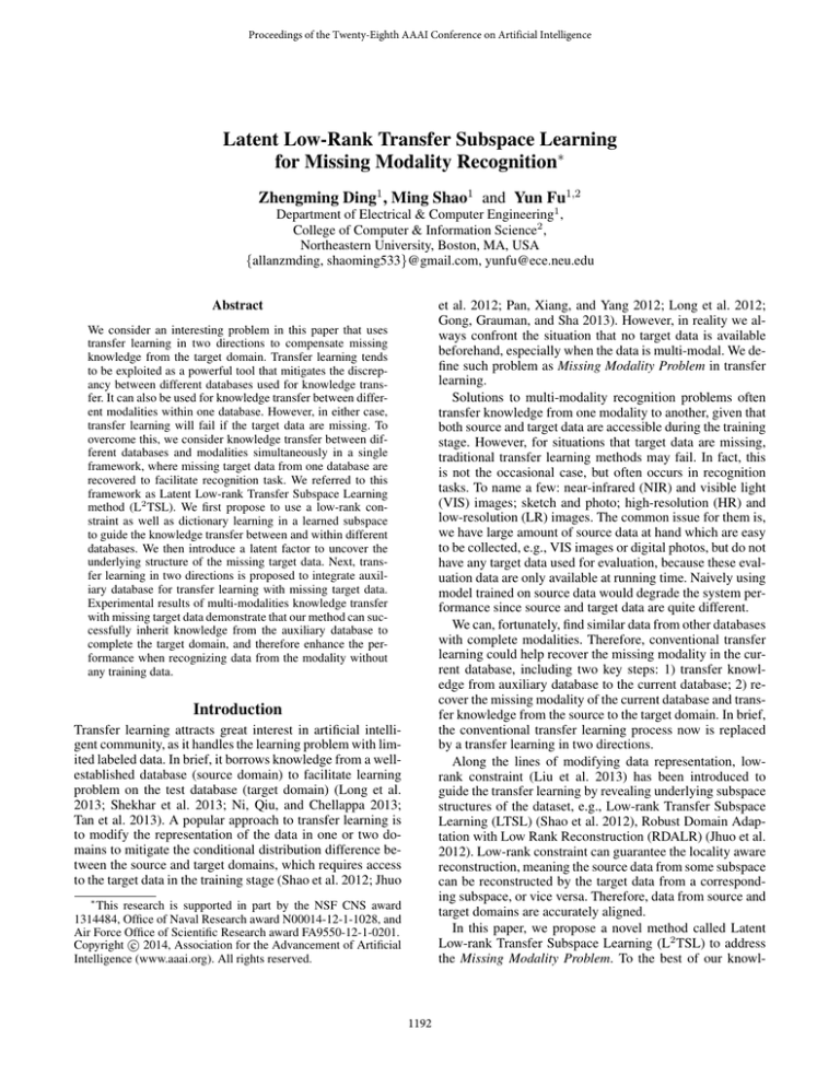
Missing Modality
Figure 1: Framework of the proposed algorithm. By introducing an auxiliary database A, we can transfer knowledge
from A to B to recover the missing modality in B. Note
same shape means data in the same database, same color
data from the same modality, T(M) transfer between modalities, and T(D) transfer between databases.
edge, this is the first time that the Missing Modality Problem
is considered under the transfer learning framework. The
core idea of L2 TSL is to learn appropriate subspaces such
that knowledge can be successfully transferred between different modalities and between two databases by a low-rank
constraint. Our main contributions are summarized as follows:
• A novel transfer learning framework (Figure 1) is proposed to handle the Missing Modality Problem. With the
auxiliary database having the same modalities, our algorithm can learn the low-dimensional subspaces from
knowledge transfer in two directions.
• A latent factor is incorporated to uncover the missing
modality with the existing data under the low-rank transfer framework. Latent information of both class structure
and modality is transferred in two directions to assist with
recognition of missing modality.
• A dictionary learning framework is introduced to couple
the knowledge from the two domains, which guarantees
the common intrinsic information between two domains
are well preserved in the learned subspace.
Related Work
Transfer learning has been widely discussed recently and
for the survey of state-of-the-art methods, please refer to
(Pan and Yang 2010). In this paper, we are more interested in transductive transfer learning: a category of transfer learning with the similar learning task, but different data
domains(Pan and Yang 2010). Specifically, along the lines
of adapting data representation, previous transductive transfer learning methods (Si, Tao, and Geng 2010; Guo 2013;
Fernando et al. 2013; Shekhar et al. 2013) learn a subspace,
or a set of subspaces, to mitigate the divergence of source
and target domains. This brings in two benefits: first, it can
avoid the curse of dimensionality (Duda, Hart, and Stork
2012) introduced by the high dimensionality of the data; second, in the common subspace, transfer learning algorithm
can align data from different domains easily. In this paper,
Latent Low-Rank Transfer Subspace Learning
Given two databases {XS , XT }, both with two modalities XS = [XS·A , XS·B ] and XT = [XT·A , XT·B ]. Traditional transfer learning is interested in problem between
different modalities such as: XS·A →XT·A or XS·B →XT·B ,
or between different databases such as: XS·A →XS·B or
XT·A →XT·B . However, when the target data is incomplete,
e.g., XT·B is missing, how can we discover the lost information of XT·B ? This is a challenging problem involving two
databases and two modalities simultaneously, which cannot
be directly solved by existing transfer learning framework.
1193
Recovering Latent Factor
ܺୱ
To address the Missing Modality Problem, we first project
both source data XS and target data XT into some common
subspace P that allows XS and XT to be aligned by lowrank constraint. Suppose projection P is known, both XS
and XT are clean, and XT·B is observable, then the lowrank transfer subspace learning can be written as:
e ∗ , s.t. P T X S = P T XT Z.
e
min kZk
(1)
Low-rank Constraint
Dictionary Constraint
ܲ୘ ܺ୘
ܲ
ܺ୘
ଶ
୊
min F(Z, L, E) + ψtr(P T WP ),
P
(7)
s.t. L(P, Z, L, E) = 0, P T UP = I,
where we use L2,1 norm on E to make it sample specific.
ψ > 0 are parameters to balance the subspace part.
In addition, we introduce a common dictionary D on the
projected data to further couple the knowledge from two domains. As a result, the dictionary and low-rank constraint on
the projected data would work synchronously in optimizing
the common subspace. This helps uncover the underlying
structure of two domains, making our method more appropriate for the Missing Modality Problem. This process is illustrated in Figure 2, and the final objective function can be
written formally as:
min F(Z, L, E) + ψtr(P T WP ) + ϕD(P, D, S),
P
(8)
s.t. L(P, Z, L, E) = 0, P T UP = I,
where ϕ is the parameter that balances the influence of
dictionary D. S represents sparse coefficients in dictionary
learning.
e
Z
According to Theorem 3.1 (Liu and Yan 2011), the optimal low-rank representation Ze∗ can be computed as:
Ze∗ = VT VST = [VT·A ; VT·B ]VST ,
(3)
where VT has also been row partitioned into VT·A and VT·B .
The constrained part now can be rewritten as:
P T XS = P T XT Ze∗ = P T [XT·A , XT·B ]Ze∗
(4)
T
where L = U ΣVT·B
VT·B Σ−1 U T should also be low-rank,
as L can recover the structure of P T XT·B .
From the above deduction, it is known that even XT·B is
unobserved, we can recover it by imposing extra constraint:
Solving the Optimization Problem
To solve the above problem, we convert Eq. (8) to the following equivalent minimization problem:
min F(J, K, E) + ψtr(P T WP ) + ϕD(P, D, S),
P
(9)
s.t.L(P, Z, L, E) = 0, Z = J, L = K, P T UP = I.
To achieve better convergence for the object function, we
apply inexact augmented Lagrange multiplier (ALM) algorithm (Lin, Chen, and Ma 2010) to solve our problem, with
the augmented Lagrangian function:
F(J, K, E) + ψtr(P T WP ) + ϕD(P, D, S)+
hY1 , Z − Ji + hY3 , L − Ki + hY4 , P T UP − Ii+
(10)
hY2 , L(P, Z, L, E)i + µ2 (kL(P, Z, L, E)k2F +
kZ − Jk2F + kL − Kk2F + kP T UP − Ik2F ),
where Y1 , Y2 , Y3 , Y4 are lagrange multipliers and µ > 0 is
a penalty parameter. k · k2F is the Frobenius norm. h, i is the
inner product of matrixes. Although there are a few variables
in need of optimization in the Eq. (10), which are difficult to
be optimized jointly, we can optimize them one by one in an
iterative manner.
The detail steps of optimization are outlined in Algorithm 1. Step 1 and 2 can be solved by Singular Value
Thresholding (SVT) (Cai, Candès, and Shen 2010), and
accelerated by many methods, such as (Liu et al. 2012;
Li and Fu 2013). P is updated by Sylvester equation (Bartels
and Stewart 1972) in step 5. Step 7 is solved by the shrinkage
operator (Yang et al. 2009).
min kZk∗ +kLk∗ , s.t. P T XS = P T XT Z +LP T XS . (5)
Z, L
Therefore, the source data P T XS is reconstructed from
the column of P T XT and the row of P T XS . When the target
domain is missing some data, the row of P T XS will make
sense in reconstruction, uncovering its latent information.
Transfer Learning with Dictionary Constraint
For simplicity, we define the following three functions.
(1).L(P, Z, L, E) = P T XS − P T XT Z − LP T XS − E
(2).D(P, D, S) = minD,S kP T X − DSk2F + γkSk1
(3).F(Z, L, E) = minZ,L,E kZk∗ + kLk∗ + λkEk2,1
We next integrate the subspace learning process into the
above function. In general, subspace learning methods can
be uniformed by the following:
P
ܲ୘ ܺୗ = ܲ୘ ܺ୘ × ܼ + ‫ܲ × ܮ‬୘ ܺୗ + ‫ܧ‬
Figure 2: Schematic diagram of the general model. The
high-dimensional data X = [XS , XT ] share a common subspace P , where P T XS and P T XT are coupled by a common dictionary D(P, D, S) and a latent low-rank representation L(P, Z, L, E) = 0.
e
Z
min tr(P T WP ), s.t. P T UP = I,
ܲ୘ ܺୱ
min஽ ܲ୘ ܺ െ ‫ܵܦ‬
Assuming Eq. (1) has a unique solution, then we can derive that in subspace P , we have P T XS ⊆ span(P T XT ).
Based on this result, we derive a new form for Eq. (1).
Suppose P T [XS , XT ] = U ΣV T and V = [VS ; VT ], where
P T XS = U ΣVST , P T XT = U ΣVTT . Then we can immee Therediately deduct the constraint as U ΣVST = U ΣVTT Z.
fore, Eq. (1) can be rewritten as:
e ∗ , s.t. VST = VTT Z.
e
min kZk
(2)
= P T [XT·A , XT·B ][VT·A ; VT·B ]VST
T
VT·B VST
= P T XT·A (VT·A VST ) + U ΣVT·B
T
T
−1 T
= P XT·A Z + (U ΣVT·B VT·B Σ U )P T XS ,
ܲ
(6)
where tr(·) denotes the trace operation. W and U are different defined according to the subspace learning methods.
Realistically, the data is often corrupted, so we add an error term E. Then the objective function of the general model
can be rewritten as:
1194
the similar modality configuration compared to the objective one, but is not captured under the exact same situation.
Therefore, it is not enough to only consider the transfer information between two modalities in the auxiliary database,
as the general transfer learning algorithms do. Our proposed
algorithm allows the knowledge transfer between databases,
which can mitigate the divergence between two databases.
Meanwhile, the latent factor can well recover the missing
modality from two directions. From Figure 1, we can observe that the missing modality XT·B is more related to
XT·A with class intrinsic structure, and to XS·B with modality information. In T(M) direction, the class structure information can help uncover the latent the label and structure
information of the missing data. In T(D) direction, the complete modality information can be transferred from the auxiliary database to the objective test modality. In this way, the
learned subspaces would be better for the Missing Modality
Problem.
In different directions, we set XS = [XS·A , XS·B ], XT =
XT·A to learn the subspace PT(D) from direction T(D) to
help transfer the modality information between databases.
We also set XS = [XS·A , XT·A ], XT = XS·B to achieve the
subspace PT(M) from direction T(M), which aims to uncover the class intrinsic information within database. In our
transfer learning, PT(M) and PT(D) are updated iteratively:
first compute one direction, then learn another direction using the data embedded in the previous subspace.
Algorithm 1 Solving Problem (9) by ALM
Input: X = [XS , XT ], λ, ϕ, ψ, W, U
Initialize: P (using Eq. (6)), Z = J = 0, L = K = 0, D = I,
E = 0, Y1 = Y2 = Y3 = Y4 = 0, µ = 10−6
while not converged do
1. Fix the others and update J by
J = arg minJ µ1 kJk∗ + 12 kJ − (Z + Y1 /µ)k2F
2. Fix the others and update K by
K = arg minK µ1 kKk∗ + 21 kK − (L + Y3 /µ)k2F
3. Fix the others and update Z by
Z = (I + XST P P T XS )−1 (XST P P T XT − XST P E
−XST P LP T XT + J + (XST P Y2 − Y1 )/µ)
4. Fix the others and update L by
T
T
T
L = (P T XT XT
P − P T XS ZXT
P − EXT
P +K
T
T
T
+(Y2 XT P − Y3 )/µ)(I + P XT XT P )−1
5. Fix the others and update P by
(2ψW + ϕXX T )P + 2UP Y4 = (XT Z − XS )Y2T +
XS Y2T L + ϕXS T DT ,
P ← orthogonal(P )
6. When P is fixed, D and S can be updated via D(P, D, S).
7. Fix the others and update E by
E = arg minE µλ kEk2,1 + 21 kL(P, Z, L, E) − Y2 /µk2F
8. Update Y1 , Y2 , Y3 , Y4 , µ
9. Check the convergence conditions.
end while
output: Z, L, E, J, K, P, D, S
Complexity and Convergency
For simplicity, assume XS and XT are both m × n matrixes.
The size of dictionary D is p × l. The time-consuming components of Algorithm 1 are Step 1 to 6. The SVD computation in Step 1-2 take O(n3 ). The general multiplication each takes O(n3 ). The inverse also costs O(n3 ). Due
to having k multiplications, Step 3-4 cost (k + 1)O(n3 ).
Step 5 is Sylvester equation, which takes O(m3 ). The dictionary learning, Step 6, takes O(2m(s2 l + 2pl)), where s
is the target sparsity. Next, we theoretically demonstrate that
the proposed optimization algorithm will converge to a local
minima, and the convergence speed is affected by the perturbation caused by projections on the manifold during the
alteration projection process. We first introduce the notation
used in our proof.
Experiments
We first introduce the databases and experimental settings,
then test the proposed algorithm on convergence property.
Ultimately, comparisons of several transfer learning algorithms on two groups of multimodal databases are presented.
Datasets and Experiments Setting
Experiments are on two sets of multimodal databases: (1)
BUAA (Di, Jia, and Yunhong 2012) and OULU VIS-NIR
face databases1 ; (2) CMU-PIE2 and Yale B face databases3 .
BUAA and OULU VIS-NIR Face databases. There are
150 subjects in BUAA database and 80 subjects in Oulu
database, and each has two modalities: VIS and NIR. As for
BUAA, we randomly select 75 subjects with corresponding
VIS images as one modality, and use the left 75 subjects with
corresponding NIR images as the other modality. For Oulu,
we randomly select 40 subjects with corresponding VIS images as one modality, and the remaining 40 subjects with
corresponding NIR images as the other modality.
CMU-PIE and Yale B Face databases. We focus on two
different modalities: HR and LR in this experiment. We use
part of CMU-PIE and Yale B databases for the experiment.
For CMU-PIE, the Pose C27 with its 68 subjects is used. For
Yale B, the cropped images with its 38 subjects are used. The
HR samples are resized into 32 × 32. For LR samples, we
first resize the 32 × 32 data (HR) to 8 × 8, then resize it to
32 × 32.
Notation: PZ is the operator to calculate {L, E} using Z,
PL is the operator to calculate {Z, E} using L and PE is the
e = P † (LP T XS +
operator to calculate {Z, L} using E. Z
1
e = (P T XT Z + E)P † and E
e = P T XT Z + LP T XS .
E), L
2
P1† and P2† are the pseudo-inverses of P T XT and P T XS .
Theorem 1. kL(P, Z, L, E)k2F converges to a local minimum when P is fixed. And the asymptotical and convergence speed of {Z, L, E} will be accelerated by shrinking:
e + PZ (Z);
e
(1) k∆Z kF /kZ + ∆Z kF for Z, where ∆Z = Z
e
e
(2) k∆L kF /kL + ∆L kF for L, where ∆L = L + PL (L); (3)
e + PE (E).
e
k∆E kF /kE + ∆E kF for E, where ∆E = E
Transfer in Two Directions
1
http://www.ee.oulu.fi/∼gyzhao/
http://vasc.ri.cmu.edu/idb/html/face/
3
http://vision.ucsd.edu/∼leekc/ExtYaleDatabase/ExtYaleB.html
2
In this section, we extend the proposed model (Figure 2)
into two directions. In fact, the auxiliary database promises
1195
P
PT(M)
T(M)
recognition rate
objecvtive value
5
4
3
2
0.6
0.4
0.2
1
0
10
20
30
iterations
40
50
0
10
20
30
iterations
40
0.8
0.8
PT(D)
T(D)
0.6
0.4
0.2
Two Directions
PT(D) Direction
recognition rate
0.8
P
recognition rate
6
P
Direction
T(M)
0
5 10 15 20 25 30 35 40 45 50 55 60
50
dimension
Figure 3: Results of convergence (left) and recognition rate
(right) with different inner iterations in two directions individually. The dimensions of PT(M) and PT(D) are 50. Here
we only show the results of 50 inner iterations.
0.6
0.4
0.2
Two Directions
P
Direction
T(D)
P
Direction
T(M)
0
5 10 15 20 25 30 35 40 45 50 55 60
dimension
Figure 4: Results of PT(M) , PT(D) , and two directions with
one outer iteration. Left is PCA case and right is LDA case.
rections with one outer iteration performs better than model
in one direction. In LDA case, however, PT(M) direction between modalities achieves better results than two directions
model. This is because, in PCA case, PT(D) helps to mitigate the divergence between two databases in terms of data
distribution and transfer more modality information to the
objective database, while in LDA case, the label information in the auxiliary database may not be applicable to the
objective database. This becomes significant when the number of classes in two databases are different. Another reason
is the dimensionality of the learned subspace. Since the dimensionality is decreasing due to the orthogonality process
in each iteration, we should keep a relative larger number of
dimensionality at the beginning; otherwise, the performance
will degrade as well. However, as to LDA case, the dimensionality is restricted by the number of the class. This explains why the dimensions of subspace in two directions can
only be 30 in Figure 4 (right).
In addition, we evaluate with more than one outer iterations. Interestingly, we find one outer iteration is adequate
for better results if we tune the dimensions of PT(M) and
PT(D) during the inner iterations appropriately, as shown in
Figure 3. One reason might be that since our method is still
in the line of traditional transfer learning, one outer iteration
is equal to the whole process of traditional transfer learning methods. Another reason is that more outer iterations
yields even lower dimensionality of the learned subspace,
leading to degenerated results. Therefore, we propose to use
one outer iteration in the following comparison experiments.
In total, we have two groups of databases: BUAA&Oulu,
CMU-PIE&Yale B, and each has four datasets (two modalities from two databases). For each group of databases, we
can select one dataset out of four as the test data (missing modality) and other three as the training data. In both
groups, we randomly select one sample per subject from the
testing data as the reference data. Note, there is no overlap between the reference and testing data. We repeat this
five times using the nearest-neighbor as the classifier, and
the average results are reported. There are two groups of experiments: (1) evaluation on convergence and property of
two directions; (2) comparisons with other transfer learning algorithms. Our methods can work in two modes: Our-I
(without dictionary learning), by setting ϕ = 0; Our-II
(with dictionary learning), by setting ϕ 6= 0.
Convergence and Property of Two Directions
In this experiment, we first test the convergence and recognition results of Our-I in two directions. Here we define one
outer iteration as first to learn PT(D) , then to learn PT(M) .
This is different from the inner iteration of the model in Eq.
(10) that iteratively updates the subspace independently in
one direction. In outer iterations, the proposed transfer learning updates both subspaces in two directions at each round.
In the convergence and recognition experiments, we first
show results of different inner iterations in two directions using PCA as the subspace method. We conduct experiments
on CMU-PIE and Yale B face databases, and take HR images of CMU-PIE as the testing data. LR of CMU-PIE and
LR and HR of Yale B are used for training. The results of
convergence and recognition rate in different inner iterations
are shown in Figure 3 where both of them converge in two
directions. It is observed that the recognition rate converges
very fast in the first several iterations, so in practice, we
choose small inner iterations (less than 20) for the following experiments. A small number of iterations also facilitates
the outer iterations as the number of independent basis of the
learned subspace in both directions is gradually decreasing
due to the orthogonalization process in updating.
Next, we show how the results were affected by the number of dimensions of the projection, and compare with our
model that transfers knowledge only in one direction. We
use the same data setting and apply two subspace learning
methods: PCA and LDA. Two directions with one outer iteration is first tested, as shown in Figure 4. In PCA, two di-
Comparison with Other Algorithms
In the second group of experiments, we compare Our-I and
Our-II with TSL (Si, Tao, and Geng 2010), LTSL(Shao et
al. 2012), RDALR(Jhuo et al. 2012), and GFK (Gong et al.
2012) in different subspace settings: PCA(Turk and Pentland
1991), LDA (Belhumeur, Hespanha, and Kriegman 1997),
Unsupervised LPP (ULPP) and Supervised LPP (SLPP) (He
and Niyogi 2004). Tables 1, 2 show the best results with optimal dimensions for 4 cases by changing training and testing data settings. Figure 5, 6 show the results in different
dimensions for one case.
It can be seen that Our-I and Our-II perform much better
than compared algorithms. Both LTSL and RDALR perform
better than TSL which demonstrates that low-rank constraint
is helpful in alignment of different domains. Compared to
LTSL and LRDAP that consider one direction knowledge
transfer, Our-I and Our-II work better. One thing is our
1196
Table 1: Best results (%) and optimal subspace dimensions of BUAA and Oulu NIR-VIS face databases, where the test data, respectively,
are NIR of BUAA (Case 1), VIS of BUAA (Case 2), NIR of Oulu (Case 3) and VIS of Oulu (Case 4).
Case 2
Case 4
ULPP
SLPP
PCA
LDA
ULPP
SLPP
PCA
LDA
ULPP
SLPP
PCA
LDA
ULPP
SLPP
35.8(70)
40.2(90)
38.3(90)
47.2(90)
52.3(80)
57.2(60)
31.3(90)
38.5(70)
12.7(39)
42.3(80)
48.7(80)
51.3(65)
29.2(80)
42.8(85)
40.2(45)
50.8(90)
59.7(70)
56.8(85)
36.8(55)
47.2(75)
39.5(60)
53.5(70)
63.7(75)
64.5(70)
37.0(60)
33.7(60)
42.3(95)
38.3(90)
49.8(80)
50.2(80)
28.3(90)
34.5(70)
15.8(35)
41.3(80)
43.2(80)
42.8(70)
38.2(90)
39.8(85)
39.2(90)
41.2(80)
49.3(70)
50.7(80)
46.8(85)
50.2(80)
48.3(90)
56.7(90)
60.7(90)
62.7(90)
39.2(60)
41.3(75)
39.5(90)
41.8(90)
48.3(80)
49.8(90)
42.2(55)
36.5(80)
26.8(70)
50.7(60)
56.8(50)
55.7(60)
47.3(70)
42.3(90)
28.3(80)
48.2(40)
50.8(90)
52.2(60)
45.7(50)
48.2(80)
45.3(80)
54.7(80)
55.7(95)
56.5(80)
31.5(90)
39.7(70)
39.2(90)
43.3(50)
46.3(90)
47.3(50)
40.3(40)
42.3(80)
38.3(60)
48.2(85)
67.5(50)
66.2(85)
39.2(60)
47.5(75)
42.8(90)
52.3(80)
58.2(90)
59.7(80)
36.2(50)
49.3(90)
29.3(85)
58.8(90)
68.5(80)
68.8(90)
0.6
0.5
0.4
0.3
0.2
0.1
0.5
0.4
0.3
0.2
0.5
0.4
0.3
0.2
0.1
0.1
0
10 20 30 40 50 60 70 80 90 100
dimension
Our−II
Our−I
0.5
0.4
0.3
0.2
0.1
0
10 20 30 40 50 60 70 80 90 100
0
10 20 30 40 50 60 70 80 90 100
dimension
0.6
0.6
0.6
recognition rate
recognition rate
Case 3
LDA
recognition rate
TSL
LRDAP
GFK
LTSL
Our-I
Our-II
Case 1
PCA
recognition rate
Methods
LTSL
GFK
0
10 20 30 40 50 60 70 80 90 100
dimension
RDALR
TSL
dimension
Figure 5: Results of six algorithms on Oulu vs. BUAA NIR-VIS face databases (Case 1) in four different subspaces. Subspace
methods from left to right are PCA, LDA, ULPP and SLPP.
Table 2: Best results (%) and optimal subspace dimensions of CMU-PIE and Yale B face databases, where the test data, respectively, are HR
of CMU-PIE (Case 1), LR of CMU-PIE (Case 2), HR of Yale B (Case 3) and LR of Yale B (Case 4).
Case 2
Case 4
ULPP
SLPP
PCA
LDA
ULPP
SLPP
PCA
LDA
ULPP
SLPP
PCA
LDA
ULPP
SLPP
22.0(60)
42.1(40)
17.3(20)
56.3(65)
60.8(65)
61.3(55)
9.1(N/A)
42.8(50)
12.3(30)
60.1(50)
74.5(30)
73.1(40)
22.2(60)
44.5(60)
40.2(35)
49.2(35)
59.5(55)
60.2(45)
22.8(55)
48.3(55)
52.8(55)
49.7(50)
62.6(55)
63.5(55)
20.3(60)
42.8(30)
17.3(30)
47.8(35)
53.2(35)
54.8(35)
50.8(50)
47.8(45)
24.1(30)
54.5(40)
60.3(60)
62.5(45)
27.4(60)
50.1(55)
23.4(40)
56.7(35)
58.4(45)
59.7(40)
48.7(50)
47.3(50)
49.8(40)
53.2(45)
54.5(50)
54.2(45)
25.4(40)
38.3(45)
8.3(N/A)
40.4(45)
41.3(50)
42.4(40)
8.2(N/A)
38.9(40)
11.2(30)
43.2(35)
45.1(40)
47.2(50)
35.3(55)
38.5(60)
40.7(60)
39.3(55)
42.2(50)
43.3(50)
35.5(45)
37.4(35)
37.8(50)
38.4(60)
43.4(50)
45.4(55)
20.0(55)
42.3(40)
8.3(30)
32.1(30)
38.4(55)
37.1(35)
21.3(55)
42.9(50)
27.8(15)
35.6(50)
37.8(30)
37.6(50)
15.2(20)
45.1(60)
33.3(60)
37.8(35)
41.6(55)
42.2(45)
20.3(50)
47.8(55)
32.2(50)
36.7(45)
41.3(35)
43.2(50)
0.8
0.6
recognition rate
recognition rate
Case 3
LDA
0.4
0.2
0.8
0.8
0.7
0.7
0.6
0.6
0.5
0.4
0.3
0.2
0.1
0
5 10 15 20 25 30 35 40 45 50 55 60
dimension
0.8
recognition rate
TSL
LRDAP
GFK
LTSL
Our-I
Our-II
Case 1
PCA
recognition rate
Methods
0.5
0.4
0.3
0.2
0.6
0.4
0.2
0.1
0
5 10 15 20 25 30 35 40 45 50 55 60
dimension
Our−II
Our−I
LTSL
0
5 10 15 20 25 30 35 40 45 50 55 60
GFK
dimension
RDALR
TSL
0
5 10 15 20 25 30 35 40 45 50 55 60
dimension
Figure 6: Results of six algorithms on CMU-PIE vs. Yale B face databases (Case 1) in four different subspaces. Subspace
methods from left to right are: PCA, LDA, ULPP and SLPP.
Conclusion
method can compensate missing modality from one database
to another, which is also helpful in knowledge transfer between modalities in the same database. In LDA case, our
method only learns the subspace in one direction between
modalities, but still achieves good performance. We attribute
this to the latent factor from the source data which uncovers
the missing information of the testing data. Furthermore, we
can see that Our-II performs better than Our-I in most cases.
This concludes that the dictionary constraint is also useful in
finding common subspace suitable for the missing modality,
as it can accurately align two domains.
In this paper, we proposed a novel Latent Low-rank Transfer Subspace Learning (L2 TSL) algorithm for the Missing
Modality Problem. With the auxiliary database, our algorithm is capable of transferring knowledge in two directions,
between modalities within one database and between two
databases. By introducing a dictionary and latent low-rank
constraints, our algorithm can learn appropriate subspaces to
better recover the missing information of the testing modality. Experiments on two groups of multimodal databases
have shown that our method can better tackle the missing
modality problem in knowledge transfer, compared to several existing transfer learning methods.
1197
References
sentation. IEEE Transactions on Pattern Analysis and Machine Intelligence 35(1):171–184.
Liu, G.; Lin, Z.; and Yu, Y. 2010. Robust subspace segmentation by low-rank representation. In 27th International
Conference on Machine Learning, 663–670.
Long, M.; Wang, J.; Ding, G.; Shen, D.; and Yang, Q. 2012.
Transfer learning with graph co-regularization. In 25th AAAI
Conference on Artificial Intelligence, 1033–1039.
Long, M.; Wang, J.; Ding, G.; Sun, J.; and Yu, P. S. 2013.
Transfer feature learning with joint distribution adaptation.
In IEEE International Conference on Computer Vision,
2200–2207.
Ni, J.; Qiu, Q.; and Chellappa, R. 2013. Subspace interpolation via dictionary learning for unsupervised domain adaptation. In IEEE Conference on Computer Vision and Pattern
Recognition, 692–699.
Pan, S. J., and Yang, Q. 2010. A survey on transfer learning. IEEE Transactions on Knowledge and Data Engineering 22(10):1345–1359.
Pan, Y.; Lai, H.; Liu, C.; Tang, Y.; and Yan, S. 2013. Rank
aggregation via low-rank and structured-sparse decomposition. In 26th AAAI Conference on Artificial Intelligence,
760–766.
Pan, W.; Xiang, E. W.; and Yang, Q. 2012. Transfer learning
in collaborative filtering with uncertain ratings. In 25th AAAI
Conference on Artificial Intelligence, 662–668.
Shao, M.; Castillo, C.; Gu, Z.; and Fu, Y. 2012. Low-rank
transfer subspace learning. In IEEE 12th International Conference on Data Mining, 1104–1109.
Shekhar, S.; Patel, V. M.; Nguyen, H. V.; and Chellappa, R.
2013. Generalized domain-adaptive dictionaries. In IEEE
Conference on Computer Vision and Pattern Recognition,
361–368.
Si, S.; Tao, D.; and Geng, B. 2010. Bregman divergence -based regularization for transfer subspace learning.
IEEE Transactions on Knowledge and Data Engineering
22(7):929–942.
Tan, B.; Xiang, E. W.; Zhong, E.; and Yang, Q. 2013. Multitransfer: Transfer learning with multiple views and multiple
sources. In SIAM International Conference on Data Mining.
Turk, M., and Pentland, A. 1991. Eigenfaces for recognition.
Journal of cognitive neuroscience 3(1):71–86.
Wang, S.; Zhang, L.; Liang, Y.; and Pan, Q. 2012.
Semi-coupled dictionary learning with applications to image super-resolution and photo-sketch synthesis. In IEEE
Conference on Computer Vision and Pattern Recognition,
2216–2223.
Yang, J.; Yin, W.; Zhang, Y.; and Wang, Y. 2009. A fast algorithm for edge-preserving variational multichannel image
restoration. SIAM Journal on Imaging Sciences 2(2):569–
592.
Zhuang, Y.; Wang, Y.; Wu, F.; Zhang, Y.; and Lu, W. 2013.
Supervised coupled dictionary learning with group structures for multi-modal retrieval. In 27th AAAI Conference
on Artificial Intelligence, 1070–1076.
Bartels, R. H., and Stewart, G. 1972. Solution of the matrix equation ax+ xb= c [f4]. Communications of the ACM
15(9):820–826.
Belhumeur, P. N.; Hespanha, J. P.; and Kriegman, D. J. 1997.
Eigenfaces vs. fisherfaces: Recognition using class specific
linear projection. IEEE Transactions on Pattern Analysis
and Machine Intelligence 19(7):711–720.
Cai, J.-F.; Candès, E. J.; and Shen, Z. 2010. A singular
value thresholding algorithm for matrix completion. SIAM
Journal on Optimization 20(4):1956–1982.
Di, H.; Jia, S.; and Yunhong, W. 2012. The buaa-visnir face
database instructions. In IRIP-TR-12-FR-001.
Duda, R. O.; Hart, P. E.; and Stork, D. G. 2012. Pattern
classification. John Wiley & Sons.
Fernando, B.; Habrard, A.; Sebban, M.; Tuytelaars, T.; et al.
2013. Unsupervised visual domain adaptation using subspace alignment. In IEEE International Conference on Computer Vision, 2960–2967.
Gong, B.; Shi, Y.; Sha, F.; and Grauman, K. 2012. Geodesic
flow kernel for unsupervised domain adaptation. In IEEE
Conference on Computer Vision and Pattern Recognition,
2066–2073.
Gong, B.; Grauman, K.; and Sha, F. 2013. Reshaping visual datasets for domain adaptation. In Advances in Neural
Information Processing Systems, 1286–1294.
Guo, Y. 2013. Robust transfer principal component analysis
with rank constraints. In Advances in Neural Information
Processing Systems, 1151–1159.
He, X., and Niyogi, P. 2004. Locality preserving projections. In Advances in Neural Information Processing Systems, 234–241.
Huang, D.-A., and Wang, Y.-C. F. 2013. Coupled dictionary and feature space learning with applications to crossdomain image synthesis and recognition. In IEEE International Conference on Computer Vision, 2496–2503.
Jhuo, I.-H.; Liu, D.; Lee, D.; and Chang, S.-F. 2012. Robust
visual domain adaptation with low-rank reconstruction. In
IEEE Conference on Computer Vision and Pattern Recognition, 2168–2175.
Li, S., and Fu, Y. 2013. Low-rank coding with b-matching
constraint for semi-supervised classification. In International Joint Conferences on Artificial Intelligence, 1472–
1478.
Lin, Z.; Chen, M.; and Ma, Y. 2010. The augmented lagrange multiplier method for exact recovery of corrupted
low-rank matrices. Technique Report, UIUC.
Liu, G., and Yan, S. 2011. Latent low-rank representation
for subspace segmentation and feature extraction. In IEEE
International Conference on Computer Vision, 1615–1622.
Liu, R.; Lin, Z.; De la Torre, F.; and Su, Z. 2012. Fixed-rank
representation for unsupervised visual learning. In IEEE
Conference on Computer Vision and Pattern Recognition,
598–605.
Liu, G.; Lin, Z.; Yan, S.; Sun, J.; Yu, Y.; and Ma, Y. 2013.
Robust recovery of subspace structures by low-rank repre-
1198