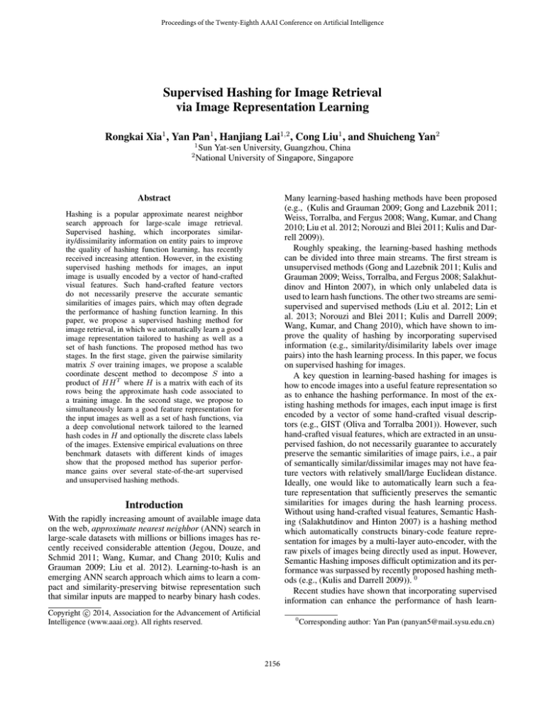
Proceedings of the Twenty-Eighth AAAI Conference on Artificial Intelligence
Supervised Hashing for Image Retrieval
via Image Representation Learning
Rongkai Xia1 , Yan Pan1 , Hanjiang Lai1,2 , Cong Liu1 , and Shuicheng Yan2
1
2
Sun Yat-sen University, Guangzhou, China
National University of Singapore, Singapore
Abstract
Many learning-based hashing methods have been proposed
(e.g., (Kulis and Grauman 2009; Gong and Lazebnik 2011;
Weiss, Torralba, and Fergus 2008; Wang, Kumar, and Chang
2010; Liu et al. 2012; Norouzi and Blei 2011; Kulis and Darrell 2009)).
Roughly speaking, the learning-based hashing methods
can be divided into three main streams. The first stream is
unsupervised methods (Gong and Lazebnik 2011; Kulis and
Grauman 2009; Weiss, Torralba, and Fergus 2008; Salakhutdinov and Hinton 2007), in which only unlabeled data is
used to learn hash functions. The other two streams are semisupervised and supervised methods (Liu et al. 2012; Lin et
al. 2013; Norouzi and Blei 2011; Kulis and Darrell 2009;
Wang, Kumar, and Chang 2010), which have shown to improve the quality of hashing by incorporating supervised
information (e.g., similarity/disimilarity labels over image
pairs) into the hash learning process. In this paper, we focus
on supervised hashing for images.
A key question in learning-based hashing for images is
how to encode images into a useful feature representation so
as to enhance the hashing performance. In most of the existing hashing methods for images, each input image is first
encoded by a vector of some hand-crafted visual descriptors (e.g., GIST (Oliva and Torralba 2001)). However, such
hand-crafted visual features, which are extracted in an unsupervised fashion, do not necessarily guarantee to accurately
preserve the semantic similarities of image pairs, i.e., a pair
of semantically similar/dissimilar images may not have feature vectors with relatively small/large Euclidean distance.
Ideally, one would like to automatically learn such a feature representation that sufficiently preserves the semantic
similarities for images during the hash learning process.
Without using hand-crafted visual features, Semantic Hashing (Salakhutdinov and Hinton 2007) is a hashing method
which automatically constructs binary-code feature representation for images by a multi-layer auto-encoder, with the
raw pixels of images being directly used as input. However,
Semantic Hashing imposes difficult optimization and its performance was surpassed by recently proposed hashing methods (e.g., (Kulis and Darrell 2009)). 0
Recent studies have shown that incorporating supervised
information can enhance the performance of hash learn-
Hashing is a popular approximate nearest neighbor
search approach for large-scale image retrieval.
Supervised hashing, which incorporates similarity/dissimilarity information on entity pairs to improve
the quality of hashing function learning, has recently
received increasing attention. However, in the existing
supervised hashing methods for images, an input
image is usually encoded by a vector of hand-crafted
visual features. Such hand-crafted feature vectors
do not necessarily preserve the accurate semantic
similarities of images pairs, which may often degrade
the performance of hashing function learning. In this
paper, we propose a supervised hashing method for
image retrieval, in which we automatically learn a good
image representation tailored to hashing as well as a
set of hash functions. The proposed method has two
stages. In the first stage, given the pairwise similarity
matrix S over training images, we propose a scalable
coordinate descent method to decompose S into a
product of HH T where H is a matrix with each of its
rows being the approximate hash code associated to
a training image. In the second stage, we propose to
simultaneously learn a good feature representation for
the input images as well as a set of hash functions, via
a deep convolutional network tailored to the learned
hash codes in H and optionally the discrete class labels
of the images. Extensive empirical evaluations on three
benchmark datasets with different kinds of images
show that the proposed method has superior performance gains over several state-of-the-art supervised
and unsupervised hashing methods.
Introduction
With the rapidly increasing amount of available image data
on the web, approximate nearest neighbor (ANN) search in
large-scale datasets with millions or billions images has recently received considerable attention (Jegou, Douze, and
Schmid 2011; Wang, Kumar, and Chang 2010; Kulis and
Grauman 2009; Liu et al. 2012). Learning-to-hash is an
emerging ANN search approach which aims to learn a compact and similarity-preserving bitwise representation such
that similar inputs are mapped to nearby binary hash codes.
c 2014, Association for the Advancement of Artificial
Copyright Intelligence (www.aaai.org). All rights reserved.
0
2156
Corresponding author: Yan Pan (panyan5@mail.sysu.edu.cn)
Figure 1: Overview of the proposed two-stage method. In stage 1, the pairwise similarity matrix S is decomposed into a product HH T ,
where H is a matrix of approximate target hash codes. In stage 2, we use a convolutional network to learn the feature representation for the
images as well as a set of hash functions. The network consists of three convolution-pooling layers, a fully connected layer and an output
layer. The output layer can be simply constructed with the learned hash codes in H (the red nodes). If the image tags are available in training,
one can add them in the output layer (the black nodes) so as to help to learn a better shared representation of the images. By inputting an test
image to the trained network, one can obtain the desired hash code from the values of the red nodes in the output layer.
ing (Liu et al. 2012; Norouzi and Blei 2011; Kulis and Darrell 2009). In this paper, we propose a supervised hashing
method for image retrieval which simultaneously learns a
set of hashing functions as well as a useful image representation tailored to the hashing task. Given n images I =
{I1 , I2 , ..., In } and a pairwise similarity matrix S in which
Si,j = 1 if Ii and Ij are semantically similar and otherwise
Si,j = −1, the task of supervised hashing is to learn a set
of q hash functions based on S and I. Formulating the hash
learning task as a single optimization problem usually leads
to a complex and highly non-convex objective which may
be difficult to optimize. To avoid this issue, one of the popular ways is decomposing the learning process into a hash
code learning stage followed by a hash function learning
stage (e.g., (Zhang et al. 2010; Lin et al. 2013)). As shown in
Figure 1, the proposed method also adopts such a two-stage
paradigm. In the first stage, we propose a scalable coordinate descent algorithm to approximately decompose S into
a product form S ≈ 1q HH T , where H ∈ Rn×q with each
of its elements being in {−1, 1}. The k-th row in H is regarded as the approximate target hash code of the image Ik .
In the second stage, we simultaneously learn a set of q hash
functions and a feature representations for the images in I
by deep convolutional neural networks (LeCun et al. 1998;
Krizhevsky, Sutskever, and Hinton 2012).
We evaluate the proposed method on several benchmark
datasets with different kinds of images. Experimental results
show that the proposed method has superior performance
gains over several state-of-the-art supervised and unsupervised hashing methods, and the proposed coordinate descent
algorithm in stage 1 performs substantially faster than the
most related competitor.
The early research of hashing focuses on dataindependent methods, in which the Locality Sensitive Hashing (LSH) methods (Gionis, Indyk, and Motwani 1999;
Charikar 2002) are the most well-known representatives.
LSH methods use simple random projections as hash functions, which are independent of the data. However, LSH
methods usually require long hash codes to achieve satisfactory search accuracies, resulting in large space for storage
and low recall in search (Liu et al. 2012).
Compared to the data-independent methods, datadependent hashing methods (as known as learning-based
hashing) aim to generate similarity-preserving representations with shorter hash codes, by learning a set of hash functions from the training data. Such compact representations
are beneficial to save space in storing large number of samples. Data-dependent methods can be divided into unsupervised, semi-supervised and supervised methods.
Unsupervised methods only use unlabeled data to generate hash functions which seek to preserve some metric distance neighbors (e.g., the `2 distance neighbors). Kernelized
LSH (Kulis and Grauman 2009), ITQ (Gong and Lazebnik
2011), SH (Weiss, Torralba, and Fergus 2008) and AGH (Liu
et al. 2011) are some representatives in this stream.
Semi-supervised or supervised methods try to improve
the quality of hashing by leveraging supervised information (e.g., pairwise labels to indicate semantic similarities
over entity pairs) into the learning process. KSH (Liu et al.
2012), BRE (Kulis and Darrell 2009), MLH (Norouzi and
Blei 2011), CGHash (Li et al. 2013), ITQ-CCA (Gong and
Lazebnik 2011) and SSH (Wang, Kumar, and Chang 2010)
are some representatives.
Most of the existing hashing methods for images first
encode each input image by hand-crafted visual features,
which may often degrade their hashing performance because
hand-crafted features do not necessarily capture accurate
similarity of the images. To tackle this issue, we propose
a supervised hashing method to simultaneously learns a set
of hash functions and a useful image feature representation
which is expected to preserve the semantic similarities of
image pairs. As can be seen in our experiments, such an automatically learned image representation shows its effectiveness in improving the hashing accuracies.
Related Work
Hashing is a widely used approach for ANN search in largescale image retrieval, due to its encouraging efficiency in
both speed and storage. Many hashing methods have been
proposed (Kulis and Grauman 2009; Gong and Lazebnik
2011; Weiss, Torralba, and Fergus 2008; Wang, Kumar,
and Chang 2010; Liu et al. 2012; Norouzi and Blei 2011;
Kulis and Darrell 2009).
2157
Without using hand-crafted features, Semantic Hashing (Salakhutdinov and Hinton 2007) learns binary-code
representation for images by stacked Restricted Boltzmanne
Machines (RBMs), with raw image pixels being as input.
However, Semantic Hashing imposes complex and difficult
optimization and its performance was surpassed by recent
hashing methods (Kulis and Darrell 2009).
Similar to the two-step paradigm in TSH (Lin et al. 2013),
the proposed method decomposes the learning process into
a hash code learning step and a hash function learning step.
However, compared to TSH, the proposed method has two
advantages: (1) We propose to solve the approximate hash
code learning problem by a coordinate descent method,
which is empirically much faster than the corresponding
decomposition method used in TSH. (2) In contrast to the
hand-crafted features used in TSH, we propose to learn hash
functions while simultaneously training a useful feature representation for the input images.
It is difficult to directly optimize (2) due to the integer
constraints on H. A natural way to relaxing the objective in
n×q
(2) is replacing H ∈ {−1, 1}
by the range constraints
n×q
H ∈ [−1, 1]
:
min ||S −
H
Input: a pairwise similarity matrix S ∈ {−1, 1}n×n , the number of bits q in a target hash code, the tolerance error , maximum
iterations T .
Initialize: randomly initialize H ∈ [−1, 1]n×q ; L ← HH T −
qS, t ← 0, F(0) ← ||L||2F , H(0) ← H, L(0) ← L.
for t=1,...,T do
Decide the order of n × q indices (i,j) by random permutation
(i=1,...,n, j=1,...,q).
for each of the n × q indices (i,j) do
Select the entry hij to update.
Calculate g 0 (Hij ) and g 00 (Hij ) by (7).
Calculate d by (6) and update Hij by Hij ← Hij + d.
Update L by (8).
end for
t ← t + 1, F(t) ← ||L||2F .
if F(t) ≤ F(t−1) then H(t) ← H, L(t) ← L,
else H(t) ← H(t−1) , L(t) ← L(t−1) , continue.
F
−Ft
if the relatively change t−1
≤ , then break.
Ft−1
end for
Output: the sign matrix of H, each of whose elements is either
1 or -1.
Given n images I = {I1 , I2 , ..., In } and a pairwise similarity matrixS defined by:
+1,
−1,
Ii , Ij are semantically similar
Ii , Ij are semantically dissimilar.
(1)
The task of supervised hashing is to learn a set of q hash
functions based on S and I.
In some supervised hashing methods, the learning task is
formulated as a single optimization objective which is complex and difficult to solve. While in other methods (Zhang
et al. 2010; Lin et al. 2013), the learning process is decomposed into two stages: a hash code learning stage followed
by a hash function learning stage, where the corresponding
optimization problems in each stage is relatively simple. The
proposed method follows the two-stage paradigm.
It is still challenging to optimize (3) due to the non-convex
term HH T . Here we propose to solve it by a coordinate descent algorithm using Newton directions. This algorithm sequentially or randomly chooses one entry in H to update
while keeping other entries fixed.
Specifically, in each iteration, we update only one entry
(i.e., Hij ) in H with other entries being fixed. Let H =
[H·1 , H·2 , . . . , H·q ], where H·j is the j-th column in H. The
objective in (3) can be rewritten as:
Stage 1: learning approximate hash codes
We define an n by q binary matrix H whose k-th row is
Hk· ∈ {−1, 1}q . Hk· represents the target q-bit hash code
for the image Ik . The goal of supervised hashing is to generate hash codes that preserve the semantic similarities over
image pairs. Specifically, the Hamming distance between
two hash codes Hi· and Hj. (associated to Ii and Ij , respectively) is expected to be correlated with Sij which indicates the semantic similarity of Ii and Ij . Existing studies (Liu et al. 2012) have pointed out that the code inner
product Hi· Hj.T has one-to-one correspondence to the Hamming distance between Hi· and Hj. . Since Hi· ∈ {−1, 1}q ,
the code inner product Hi· Hj.T is in the range [−q, q]. Hence,
as shown in Figure 1(Stage 1), we learn the approximate
hash codes for the training images in I by minimizing the
following reconstruction errors:
n X
n
X
1
1
T 2
min
(Sij − Hi· Hj.
) = min ||S − HH T ||2F ,
H
H
q
q
i=1 j=1
(3)
Algorithm 1 Coordinate descent algorithm for hash bit
learning.
The Approach
Sij =
1
HH T ||2F s.t. H ∈ [−1, 1]n×q .
q
T
kH·j H·j
− (qS −
X
T
H·c H·c
)k2F
c6=j
T
=||H·j H·j
− R||2F =
n X
n
X
(Hlj Hkj − Rlk )2
P l=1 k=1 T
where we set R = qS − c6=j H·c H·c
. Since S is symmetric, it is easy to verify that R is also symmetric. By fixing
other entries in H, the objective w.r.t. Hij can be rewritten
as:
n
n
g(Hij ) =
XX
(Hlj Hkj − Rlk )2
l=1 k=1
2
=(Hij
(2)
− Rii )2 + 2
X
(Hij Hkj − Rik )2 + constant,
k6=i
where we use the fact that R is symmetric.
Suppose we update Hij to Hij + d, the corresponding
optimization problem is:
min g(Hij + d) s.t. − 1 ≤ Hij + d ≤ 1.
n×q
where || · ||F is the Frobenius norm and H ∈ {−1, 1}
.
For the training images, H encodes the approximate hash
codes which preserve the pairwise similarities in S. Note
that the code inner product Hi· Hj.T is divided by q in order
to fit Sij ∈ {−1, 1}.
d
To simplify the search of d, we approximate g(Hij + d)
2158
Method
CNNH+
CNNH
KSH
ITQ-CCA
MLH
BRE
SH
ITQ
LSH
12 bits
0.969
0.957
0.872
0.659
0.472
0.515
0.265
0.388
0.187
MNIST(MAP)
24 bits 32 bits
0.975
0.971
0.963
0.956
0.897
0.891
0.694
0.714
0.666
0.652
0.593
0.613
0.267
0.259
0.436
0.422
0.209
0.235
48 bits
0.975
0.960
0.900
0.726
0.654
0.634
0.250
0.429
0.243
12 bits
0.465
0.439
0.303
0.264
0.182
0.159
0.131
0.162
0.121
CIFAR10(MAP)
24 bits 32 bits
0.521
0.521
0.511
0.509
0.346
0.337
0.282
0.288
0.195
0.207
0.181
0.193
0.135
0.133
0.169
0.172
0.126
0.120
48bits
0.532
0.522
0.356
0.295
0.211
0.196
0.130
0.175
0.120
12 bits
0.623
0.611
0.556
0.435
0.500
0.485
0.433
0.452
0.403
NUS-WIDE(MAP)
24 bits 32 bits 48 bits
0.630
0.629
0.625
0.618
0.625
0.608
0.581
0.588
0.572
0.435
0.435
0.435
0.514
0.520
0.522
0.525
0.530
0.544
0.426
0.426
0.423
0.468
0.472
0.477
0.421
0.426
0.441
Table 1: MAP of Hamming ranking w.r.t different number of bits on three datasets. For NUS-WIDE, we calculate the MAP
values within the top 5000 returned neighbors. The results of CNNH / CNNH+ are the average of 5 trials.
T = 5 and q ≤ 64 in our experiments), making the algorithm scale well with relatively large n.
by a quadratic function via Taylor expansion:
ĝ(Hij + d) = g(Hij ) + g 0 (Hij )d +
1 00
g (Hij )d2 ,
2
(4)
where g 0 (Hij ) (g 00 (Hij )) is the first (second) order derivative of g at Hij :
n
X
g 0 (Hij ) = 4
(Hij Hkj − Rik )Hkj
Stage 2: learning image feature representation and
hash functions
In contrast to the existing supervised hashing methods which
use hand-crafted visual features for images, in the second
stage, we simultaneously learn a feature representation for
the training images as well as a set of hash functions.
Recently, deep learning has become a hot topic in machine learning research. In contrast to other deep architectures (e.g., (Hinton and Salakhutdinov 2006; Salakhutdinov and Hinton 2009)), deep convolutional neural networks
(CNNs) (LeCun et al. 1998) are designed to take advantage
of the 2D structure of images and able to learn translation
invariant features. CNNs have shown encouraging results in
various visual tasks such as object recognition (Krizhevsky,
Sutskever, and Hinton 2012). Here we focus on leveraging
convolutional networks in hash learning. We adopt the wellknown architecture in (Krizhevsky, Sutskever, and Hinton
2012) as our basic framework. As shown in Figure 1(Stage
2), our network has three convolution-pooling layers with
rectified linear activation, max pooling and local contrast
normalization, a standard fully connected layer and an output layer with softmax activation. We use 32, 64, 128 filters
(with the size 5 × 5) in the 1st, 2nd and 3rd convolutional
layers. We use dropout (Hinton et al. 2012) in the fully connected layer with a rate of 0.5. Here we mainly focus on the
design of the output layer, so as to explore how to train a
network tailored to the hashing task.
In many scenarios of supervised hashing for images, the
similarity/dissimilarity labels on image pairs are derived
from the discrete class labels of the individual images. That
is, in hash learning, the discrete class labels of the training
images are usually available. Here we can design the output
layer of our network in two ways, depending on whether the
discrete class labels of the training images are available.
In the first way, given only the learned hash code matrix H with each of its rows being a q-bit hash code for a
training image, we define an output layer with q output units
(the red nodes in the output layer in Figure 1(Stage 2)), each
of which corresponds to one bit in the target hash code for
an image. We denote the proposed hashing method using a
CNN with such an output layer (with only the red nodes, ignoring the black nodes and the associated lines) as CNNH.
k=1
2
g 00 (Hij ) = 12Hij
− 4Rii + 4
X
2
Hkj
k6=i
By setting the derivative of (4) w.r.t. d to be zero, we have
g 0 (H )
d = − g00 (Hijij ) . Hence, the solution to the objective
min ĝ(Hij + d) s.t. − 1 ≤ Hij + d ≤ 1.
is
d
d = max(−1 − Hij , min(−
g 0 (Hij )
, 1 − Hij )),
g 00 (Hij )
(5)
(6)
which can be used in the update rule Hij ← Hij + d.
calculating the matrix R = qS −
PNote thatTdirectlyn×n
needs O(n2 ) time, which is timec6=i H·c H·c ∈ R
consuming with large number n of training images. To
tackle this issue, we do not calculate R explicitly. Specifically, we maintain a matrix L = HH T − qS. Given L,
g 0 (Hij ) and g 00 (Hij ) can be calculated by:
T
2
g 0 (Hij ) = 4Li· H·j , g 00 (Hij ) = 4(H·j
H·j + Hij
+ Lii ), (7)
where Li· is the i-th row of L. Hence, we can calculate
g 0 (Hij ) and g 00 (Hij ) in O(n) time. After Hij is updated,
it is easy to verify that only the i-th row and i-th column
of L are affected. For example, given Hij ← Hij + d, we
update L by:
T
Li· ← Li· + dH·j
, L·i ← L·i + dH·j , Lii ← Lii + d2 .
(8)
Hence, the time complexity of updating L is also O(n).
The sketch of the proposed coordinate descent algorithm
is shown in Algorithm 11 . In each iteration of the inner loop,
the overall time complexity is O(n). The time complexity of
the whole algorithm is O(T qn2 ) with small T and q (e.g.,
1
Since the objective (3) is non-convex w.r.t. H, Algorithm 1
is a greedy algorithm and it cannot guarantee to decrease (3) in
each iteration. Hence, similar to existing methods (Liu et al. 2012;
Lin et al. 2013; Kulis and Darrell 2009), if in some iteration (of the
outer loop) increases the value of (3), Algorithm 1 does not update
H and L and continues the loop (see the IF-ELSE block in the
outer loop of Algorithm 1). Note that in our experiments, we found
that Algorithm 1 decreases (3) in every iteration.
2159
In the second way, we assume the discrete class labels of
the training images are available. Specifically, for n training images in c classes (an image may belong to multiple classes), we define a n by c discrete label matrix Y ∈
{0, 1}n×c , where Yij = 1 if the i-th training image belongs
to the j-th class, otherwise Yij = 0. For the output layer in
our network, in addition to defining the q output units (the
red nodes in the output layer) corresponding to the hash bits
as in the first way, we add c output units (the black nodes
in the output layer in Figure 1(Stage 2)) which correspond
to the class labels of a training images. By incorporating the
image class labels as a part in the output layer, we enforce
the network to learn a shared image representation which
matches both the approximate hash codes and the image
class labels. It can be regarded as a transfer learning case
in which the incorporated image class labels are expected to
be helpful for learning a more accurate image representation
(i.e. the hidden units in the fully connected layer). Such a
better image representation may be advantageous for hash
functions learning. We denote the proposed method using a
CNN with the output layer having both the red nodes and
the black nodes as CNNH+.
The convolutional networks automatically learn an image
representation (represented by the orange nodes in the fully
connected layer) as well as a set of hash functions (represented by the solid lines between the orange nodes and the
red nodes within the last two layers). In prediction, one can
input a test image to the trained networks and obtain the hash
code from the values of the red nodes in the output layer.
ods are obtained by the open-source implementations provided by their respective authors.
In MNIST and CIFAR-10, we randomly select 1K images
(100 images per class) as the test query set. For the unsupervised methods, we use the rest images as training samples.
For the supervised methods, we randomly select 5K images
(500 images per class) from the rest images as the training
set. The pairwise similarity matrix S is constructed based on
the image class labels.
In NUS-WIDE, we randomly sample 100 images from
each of the selected 21 classes to form a test query set of
2,100 images. For the unsupervised methods, the rest images
in the selected 21 classes are used as the training set. For supervised methods, we uniformly sample 500 images from
each of the selected 21 classes to form a training set. We
construct the pairwise similarity matrix S based on whether
two images share at least one common tag.
For the proposed CNNH and CNNH+, we directly use
the image pixels as input. For all of the baseline methods, we follow (Norouzi and Blei 2011; Wang, Kumar, and
Chang 2010) to represent each image in MNIST by a 784dimensional greyscale vector; we follow (Liu et al. 2012)
to represent each image in CIFAR-10 by a 512-dimensional
GIST vector; we represent each image in NUS-WIDE by a
500-dimensional bag-of-words vector (which is included in
the NUS-WIDE dataset).
To evaluate the quality of hashing, we use four evaluation
metrics: Mean Average Precision (MAP), Precision-Recall
curves, Precision curves within Hamming distance 2, and
Precision curves w.r.t. different number of top returned samples. For fair comparisons, all of the methods use identical
training and test sets.
Since CNNH and CNNH+ use random initialization of H
in stage 1, in all of the experiments, the results of CNNH
and CNNH+ are the average of 5 trials.
As shown in Table 1 and Figure 2∼4, two observations
can be made from the results:
(1) On all of the three datasets, CNNH+ and CNNH
achieve substantially better search accuracies (w.r.t. MAP,
precision within Hamming distance 2, precision-recall, and
precision with varying size of top returned samples) than
the baseline methods. For example, compared to the second best competitor (except for CNNH), the MAP results
of CNNH+ indicate a relative increase of 8.2% ∼ 11.1%
/ 49.4% ∼ 54.6% / 6.3% ∼ 12.1% on MNIST / CIFAR10 / NUS-WIDE, respectively. The substantial superior performance of CNNH+ verifies that automatically learning a
good image representation as well as a set of hash functions
is beneficial to enhance the hashing quality for images.
(2) CNNH+ shows slightly but consistently better search
accuracies than CNNH, which verifies that incorporating
both the approximate hash codes and image tags in training helps to learn a better shared image representation and
enhance the hashing performance.
Note that various hand-crafted features can be used in the
baseline methods. We conduct experiments to observe the
effects on hashing with different features. We only evaluate
KSH because it performs the best among the baselines. As
shown in Figure 6, on MNIST and CIFAR-10, the search
Experiments
Results on image search
We evaluate the proposed method on three benchmark
datasets with different kinds of images. (1) The MNIST2
dataset consists of 70K 28 × 28 greyscale images of handwritten digits from ’0’ to ’9’. (2) The CIFAR-103 consists
of 60K 32 × 32 color tinny images which are categorized
into 10 classes (6K images per class). (3) The NUS-WIDE4
dataset has nearly 270K images collected from the web. It is
a multi-label dataset in which each image is annotated with
one or multiple semantic tags (class labels) from 81 concept
tags. Following (Liu et al. 2011), we only use the images
associated with the 21 most frequent concept tags (classes),
where the number of images associated with each tag is at
least 5K. For simplicity, we resize each image to 64 × 64.
We compare the performance of the proposed CNNH and
CNNH+ against seven state-of-the-art hashing methods, including three unsupervised methods LSH (Gionis, Indyk,
and Motwani 1999), SH (Weiss, Torralba, and Fergus 2008)
and ITQ (Gong and Lazebnik 2011), and four supervised
methods KSH (Liu et al. 2012), MLH (Norouzi and Blei
2011), BRE (Kulis and Darrell 2009) and ITQ-CCA (Gong
and Lazebnik 2011). The results of LSH are obtained by our
implementation. The results of the other six baseline meth2
http://yann.lecun.com/exdb/mnist/
http://www.cs.toronto.edu/ kriz/cifar.html
4
http://lms.comp.nus.edu.sg/research/NUS-WIDE.htm
3
2160
(a)
(b)
(c)
Figure 2: The results on MNIST. (a) precision curves within Hamming radius 2; (b) precision-recall curves of Hamming ranking with 48
bits; (c) precision curves with 48 bits w.r.t. different number of top returned samples.
(a)
(b)
(c)
Figure 3: The results on CIFAR10. (a) precision curves within Hamming radius 2; (b) precision-recall curves of Hamming ranking with 48
bits; (c) precision curves with 48 bits w.r.t. different number of top returned samples
(a)
(b)
(c)
Figure 4: The results on NUS-WIDE. (a) precision curves within Hamming radius 2; (b) precision-recall curves of Hamming ranking with
48 bits; (c) precision curves with 48 bits w.r.t. different number of top returned samples
accuracies of KSH with raw pixels, 512-dim GIST, 1024dim GIST and 21504-dim sparse-coding features (extracted
by LLC (Wang et al. 2010)) are inferior to those of CNNH+.
Automatically learning features in CNNH+ makes it easy to
be applied to image retrieval in new domains.
(a)
(b)
Figure 6: Comparison results of KSH with different features on
(a) CIFAR-10, and (b) MNIST.
Efficiency of approximate hash code learning
(a)
In stage 1 of CNNH/CNNH+, we proposed a coordinate descent algorithm to factorize S into HH T , whose time complexity is O(T qn2 ). Note that there exist other algorithms to
(b)
Figure 5: CPU time of stage 1 on CIFAR10.
2161
factorize S into HH T , such as the block coordinate descent
(BCD) algorithm in (Lin et al. 2013). Hence, we empirically
compare the efficiency of the propose coordinate descent algorithm to the most related BCD algorithm in (Lin et al.
2013)5 on CIFAR-10. For fair comparisons, we use the same
stopping criterion (as shown in Algorithm 1) in the two algorithms. As can be seen in Figure 5, the proposed coordinate
descent algorithm is much faster to converge than the BCD
algorithm. For either the number n of training samples or the
number q of bits increasing, the CPU time of the baseline
increases more rapidly than the proposed algorithm, which
indicates the proposed algorithm’s superior scalability in the
scenarios with large number of training samples.
Krizhevsky, A.; Sutskever, I.; and Hinton, G. 2012. Imagenet
classification with deep convolutional neural networks. In Proceedings of Advances in Neural Information Processing Systems, 1106–1114.
Kulis, B., and Darrell, T. 2009. Learning to hash with binary
reconstructive embeddings. In Proceedings of the Advances in
Neural Information Processing Systems, 1042–1050.
Kulis, B., and Grauman, K. 2009. Kernelized locality-sensitive
hashing for scalable image search. In Proceedings of the IEEE
International Conference on Computer Vision, 2130–2137.
LeCun, Y.; Bottou, L.; Bengio, Y.; and Haffner, P. 1998.
Gradient-based learning applied to document recognition. Proceedings of the IEEE 86(11):2278–2324.
Li, X.; Lin, G.; Shen, C.; Hengel, A. v. d.; and Dick, A. 2013.
Learning hash functions using column generation. In Proceedings of the International Conference on Machine Learning.
Lin, G.; Shen, C.; Suter, D.; and van den Hengel, A. 2013. A
general two-step approach to learning-based hashing. In Proceedings of the IEEE Conference on Computer Vision.
Liu, W.; Wang, J.; Kumar, S.; and Chang, S.-F. 2011. Hashing
with graphs. In Proceedings of the International Conference
on Machine Learning, 1–8.
Liu, W.; Wang, J.; Ji, R.; Jiang, Y.-G.; and Chang, S.-F.
2012. Supervised hashing with kernels. In Proceedings of
the IEEE Conference on Computer Vision and Pattern Recognition, 2074–2081.
Norouzi, M., and Blei, D. M. 2011. Minimal loss hashing
for compact binary codes. In Proceedings of the International
Conference on Machine Learning, 353–360.
Oliva, A., and Torralba, A. 2001. Modeling the shape of the
scene: A holistic representation of the spatial envelope. International Journal of Computer Vision 42(3):145–175.
Salakhutdinov, R., and Hinton, G. 2007. Learning a nonlinear
embedding by preserving class neighbourhood structure. In
Proceedings of the International Conference on Artificial Intelligence and Statistics, volume 11.
Salakhutdinov, R., and Hinton, G. E. 2009. Deep boltzmann
machines. In Proceedings of the International Conference on
Artificial Intelligence and Statistics, 448–455.
Wang, J.; Yang, J.; Yu, K.; Lv, F.; Huang, T.; and Gong, Y.
2010. Locality-constrained linear coding for image classification. In Proceedings of the IEEE Conference on Computer
Vision and Pattern Recognition, 3360–3367.
Wang, J.; Kumar, S.; and Chang, S.-F. 2010. Semi-supervised
hashing for scalable image retrieval. In Proceedings of the
IEEE Conference on Computer Vision and Pattern Recognition, 3424–3431.
Weiss, Y.; Torralba, A.; and Fergus, R. 2008. Spectral hashing. In Proceedings of the Advances in Neural Information
Processing Systems, 1753–1760.
Zhang, D.; Wang, J.; Cai, D.; and Lu, J. 2010. Self-taught
hashing for fast similarity search. In Proceedings of the International ACM SIGIR Conference on Research and Development in Information Retrieval, 18–25.
Conclusions
In this paper, we developed a supervised hashing method
for image retrieval, which simultaneously learns a good representation of images as well as a set of hash functions.
The proposed method firstly factorizes the pairwise semantic
similarity matrix into approximate hash codes for the training images, and then trains a deep convolutional network
with the approximate hash codes as well as the image tags (if
available). Empirical evaluations in image search show that
the proposed method has encouraging performance gains
over state-of-the-arts.
Acknowledgment
This work was funded in part by National Science Foundation of China (grant No. 61370021, 61003045, 61003241),
Natural Science Foundation of Guangdong Province, China
(grant No. S2013010011905). Yan Pan is the corresponding
author of this paper (panyan5@mail.sysu.edu.cn).
References
Charikar, M. S. 2002. Similarity estimation techniques from
rounding algorithms. In Proceedings of the Annual ACM Symposium on Theory of Computing, 380–388.
Gionis, A.; Indyk, P.; and Motwani, R. 1999. Similarity search
in high dimensions via hashing. In Proceedings of the International Conference on Very Large Data Bases, volume 99,
518–529.
Gong, Y., and Lazebnik, S. 2011. Iterative quantization: A
procrustean approach to learning binary codes. In Proceedings of the IEEE Conference on Computer Vision and Pattern
Recognition, 817–824.
Hinton, G. E., and Salakhutdinov, R. R. 2006. Reducing
the dimensionality of data with neural networks. Science
313(5786):504–507.
Hinton, G. E.; Srivastava, N.; Krizhevsky, A.; Sutskever, I.; and
Salakhutdinov, R. R. 2012. Improving neural networks by
preventing co-adaptation of feature detectors. arXiv preprint
arXiv:1207.0580.
Jegou, H.; Douze, M.; and Schmid, C. 2011. Product quantization for nearest neighbor search. IEEE Transactions on Pattern
Analysis and Machine Intelligence 33(1):117–128.
5
We carefully implemented the BCD algorithm in (Lin
et al. 2013), in which we used the LBFGS-B solver at
http://users.eecs.northwestern.edu/ nocedal/lbfgsb.html.
2162