Proceedings of the Twenty-Seventh AAAI Conference on Artificial Intelligence
Basis Adaptation for Sparse Nonlinear Reinforcement Learning
Sridhar Mahadevan, Stephen Giguere, and Nicholas Jacek
School of Computer Science
University of Massachusetts, Amherst
mahadeva@cs.umass.edu, nicolas.jacek@gmail.com, sgiguere9@gmail.com
In this paper, we present a new framework for basis adaptation as nonlinear separable least-squares approximation of
value functions using variable projection functionals. This
framework is adapted from a well-known classical method
for nonlinear regression (Golub and Pereyra 1973), when
the model parameters can be decomposed into a linear set,
which is fit by classical least-squares, and a nonlinear set,
which is fit by a Gauss-Newton method based on computing
the gradient of an error function based on variable projection
functionals.
Mirror descent is a highly scalable online convex optimization framework (Nemirovksi and Yudin 1983). Online
convex optimization (Zinkevich 2003) explores the use of
first-order gradient methods for solving convex optimization
problems. Mirror descent can be viewed as a first-order proximal gradient based method (Beck and Teboulle 2003) using
a distance generating function that is a Bregman divergence
(Bregman 1967). We combine basis adaptation with mirrordescent RL (Mahadevan and Liu 2012), a recently developed
first-order approach to sparse RL. The proposed approach
is also validated with some experiments showing improved
performance compared to previous work.
Abstract
This paper presents a new approach to representation
discovery in reinforcement learning (RL) using basis
adaptation. We introduce a general framework for basis
adaptation as nonlinear separable least-squares value
function approximation based on finding Fréchet gradients of an error function using variable projection functionals. We then present a scalable proximal gradientbased approach for basis adaptation using the recently
proposed mirror-descent framework for RL. Unlike traditional temporal-difference (TD) methods for RL, mirror descent based RL methods undertake proximal gradient updates of weights in a dual space, which is linked
together with the primal space using a Legendre transform involving the gradient of a strongly convex function. Mirror descent RL can be viewed as a proximal
TD algorithm using Bregman divergence as the distance
generating function. We present a new class of regularized proximal-gradient based TD methods, which combine feature selection through sparse L1 regularization
and basis adaptation. Experimental results are provided
to illustrate and validate the approach.
Introduction
Reinforcement Learning
There has been rapidly growing interest in reinforcement
learning in representation discovery (Mahadevan 2008). Basis construction algorithms (Mahadevan 2009) combine the
learning of features, or basis functions, and control. Basis adaptation (Bertsekas and Yu 2009; Castro and Mannor 2010; Menache, Shimkin, and Mannor 2005) enables
tuning a given parametric basis, such as the Fourier basis (Konidaris, Osentoski, and Thomas 2011), radial basis
functions (RBF) (Menache, Shimkin, and Mannor 2005),
polynomial bases (Lagoudakis and Parr 2003), etc. to the
geometry of a particular Markov decision process (MDP).
Basis selection methods combine sparse feature selection
through L1 regularization with traditional least-squares type
RL methods (Kolter and Ng 2009; Johns, Painter-Wakefield,
and Parr 2010), linear complementarity methods (Johns,
Painter-Wakefield, and Parr 2010), approximate linear programming (Petrik et al. 2010), or convex-concave optimization methods for sparse off-policy TD-learning (Liu, Mahadevan, and Liu 2012).
Reinforcement learning can be viewed as a stochastic approximation framework (Borkar 2008) for solving MDPs,
which are defined by a set of states S, a set of (possibly
state-dependent) actions A (As ), a dynamical system model
a
comprised of the transition probabilities Pss
specifying the
probability of transitioning to state s from state s under
action a, and a reward model R specifying the payoffs received. A policy π : S → A is a deterministic mapping
from states to actions. Associated with each policy π is a
value function V π , which is a fixed point of the Bellman
equation:
V π = T π (V π ) = Rπ + γP π V π
(1)
where 0 ≤ γ < 1 is a discount factor, and T π is the Bellman operator. An optimal policy π ∗ is one whose associated
value function dominates all others, and is defined by the
following nonlinear system of equations:
∗
a
a
∗ Pss
V (s) = max
(Rss + γV (s ))
c 2013, Association for the Advancement of Artificial
Copyright Intelligence (www.aaai.org). All rights reserved.
a
654
s
The optimal action value Q∗ (s, a) represents a convenient
reformulation of the optimal value function, defined as the
long-term value of performing a first, and then acting optimally according to V ∗ :
∗
Q∗ (s, a) = E rt+1 + γ max
Q
(s
,
a
)|s
=
s,
a
=
a
t+1
t
t
Nonlinear Value Function Approximation
A key contribution of this paper is a general framework for
nonlinear value function approximation based on nonlinear separable least-squares. This framework helps clarify
previously proposed algorithms (Castro and Mannor 2010;
Bertsekas and Yu 2009; Menache, Shimkin, and Mannor
2005), which amount to particular instances of this general
framework. Concretely, basis adaptation can be understood
as modifying a parameterized basis, Φ(α) where α denotes
the nonlinear parameters, and w denotes the linear parameters, such that V̂ ≈ Φ(α)w. For example, for radial basis
function (RBF) bases, α would correspond to the mean (center), μi , and covariance (width) parameters, Σi , of a fixed set
of bases, where these would be tuned based on optimizing
some particular error, such as the Bellman error (Menache,
Shimkin, and Mannor 2005). Such an approach can broadly
be characterized using the framework of separable nonlinear
least squares framework for regression (Golub and Pereyra
1973), which provides a framework for unifying past work
on basis adaptation. The general nonlinear regression problem is to estimate a vector of parameters θ from a set of
training examples D = {(x1 , y1 ), . . . , (xn , yn )} to minimize (for example) the squared error:
a
(2)
where rt+1 is the actual reward received at the next time
step, and st+1 is the state resulting from executing action
a in state st . When the set of states, S, is large, it is often necessary to approximate the value function, V , using
a set of handcrafted basis functions (e.g., polynomials, radial basis functions, wavelets etc.) or automatically generated basis functions (Mahadevan 2009). In linear value function approximation, the value function is assumed to lie in
the linear span of the basis function matrix Φ of dimension |S| × p, where it is assumed that p |S|.1 Hence,
V π ≈ V̂ π = Φw. The (optimal) action value formulation is convenient because it can be approximately solved
by a temporal-difference (TD) learning technique called Qlearning (Watkins 1989). The TD(0) rule for linear function
approximated value functions is given as:
wt+1 = wt + βt (rt + γφ(st+1 ), wt − φ(st ), wt ) φ(st )
(3)
where the quantity in the parenthesis is the TD error. TD
can be shown to converge to the fixed point of the composition of the projector ΠΦ onto the column space of Φ and the
Bellman operator T π . TD(0) converges to the value function V π for policy π as long as the samples are “on-policy”,
that is following the stochastic Markov chain associated with
the policy; and the learning rate βt is decayed according to
the Robbins-Monro
conditions
∞
∞ in stochastic approximation
theory: t=0 βt = ∞, t=0 βt2 < ∞ (Bertsekas and Tsitsiklis 1996). l1 regularized least-squares methods for solving MDPs attempt to find a fixed point of the l1 penalized
Bellman equation (Kolter and Ng 2009; Petrik et al. 2010;
Johns, Painter-Wakefield, and Parr 2010):
w = f (w) = argminu (Rπ + γP π Φw − Φu)2 + νu1
(4)
Another way to introduce l1 regularization is to penalize the
projected Bellman residual (Geist and Scherrer 2011), which
yields a convex optimization problem:
J(θ) =
=
argminw Rπ + γP π Φθ − Φw
θ∗
=
argminθ Φwθ − Φθ2 + νθ1
2
yi − f (xi ; θ)2 .
i=1
In the nonlinear separable least squares setting, the function f (xi ; θ) = f (xi ; α, w) = [Φ(α)w]i , where α are the
nonlinear variables and w denote the linear variables. The
squared error can now be written as:
J(α, w) = y − Φ(α)w2 = I − Φ(α)Φ† (α) y2
Golub and Pereyra define the last (boldfaced) term above
as the variable projection functional (VP). To explain the
derivation of the second step from the first, note that for
a specified value of the nonlinear parameters α, for the
best linear fit, the linear parameter values can computed as
ŵ = Φ† (α)y (here, † denotes the Moore-Penrose pseudoinverse). Geometrically, note that
†
Π⊥
Φ(α) = (I − Φ(α)Φ (α))
is the projector onto the complement of the column space
of the parameterized basis matrix Φ(α). Using this notation,
the nonlinear separable least squares problem can be stated
formally as:
2
wθ
n
(5)
where the first step is the projection step and the second
is the fixed point step. Recent l1 -regularized RL methods,
such as LARS-TD and LCP-TD, involve matrix inversion,
requiring at least quadratic complexity in the number of (active) features. In contrast, mirror-descent based RL methods
(Mahadevan and Liu 2012) can provide similar performance
while requiring time per step only linear in the number of
features.
If this problem is solved to find the optimal αopt , the optimal linear parameters wopt = Φ† (αopt )y. To argue that this
strategy is correct, Golub and Pereyra prove the following
result:
In practice, the full Φ matrix is never constructed, and only the
p-dimensional embeddings φ(s) of sampled states are explicitly
formed. Also, Rπ , Φ, and P π Φ are approximated by R̃, Φ̃, and Φ̃
over a given set of samples. Finally, ., . denotes the dot product.
Theorem 1 (Golub and Pereyra 1973) Assume that Φ(α)
has constant rank r in every open set Ω ⊂ Rk , where α ∈ Ω.
If (α∗ , w∗ ) is the global minimizer of J(α, w), then αopt =
α∗ and wopt = w∗ .
2
αopt = arg min Π⊥
Φ(α) y
α
1
655
(6)
Initial RBF centers
To solve the optimization problem given by Equation 6,
Golub and Pereyra derive a modified Gauss-Newton algorithm. The key step in their algorithm involves computa2
tion of the Jacobian ∇Π⊥
Φ(α) y , which involves finding
the gradient of the pseudo inverse as follows:
25
20
15
10
5
0
1
1
2
⊥
†
∇Π⊥
Φ(α) y = −y, ΠΦ(α) DΦ(α)Φ (α)y
2
where DΦ(α) is the Fréchet (or tensor) derivative of the parameterized basis matrix Φ(α). If there are m basis functions
φi (columns of Φ(α)), n training points, and k nonlinear parameters α, then DΦ(α) is a tensor of size n × m × k.
5
6
7
5
6
7
5
4
3.5
3
1
2
3
4
Final RBF centers
20
15
2ρπ
10
5
0
1
(7)
arg min Rπ + γP π V̂ − V̂ 2
=
arg min Rπ + (γP π Φ(α) − Φ(α))(Ψπα )† Rπ 2
α
arg min I − (I − γP π )Φ(α)(Ψπα )† Rπ 2
3
4
5
6
7
5
6
7
4
x2ρπ
=
2
Final RBF Widths
3.8
where V̂ = Φ(α)w ≈ V , and the norm
≡
x, Dρπ x where Dρπ is a diagonal matrix whose entries
reflect the stationary distribution of the Markov chain corresponding to policy π. To lighten the notation below, we
will assume Dρπ = I, although our entire derivation carries
through without change in the more general case.
Defining Ψπα = ((I − γP π )Φ(α)), we can now eliminate
the linear variables wN BR and write the nonlinear Bellman
residual variable projection functional as follows: αN BR =
π
=
4
4.5
Bellman Residual VP Functional
(αBR , wBR ) = argminw,α T (V̂ ) − V̂
3
Initial RBF Widths
The Nonlinear Bellman Residual minimization problem is to
find a set of nonlinear weights αBR ∈ Rk and linear weights
wBR such that2
π
2
3.6
3.4
3.2
1
2
3
4
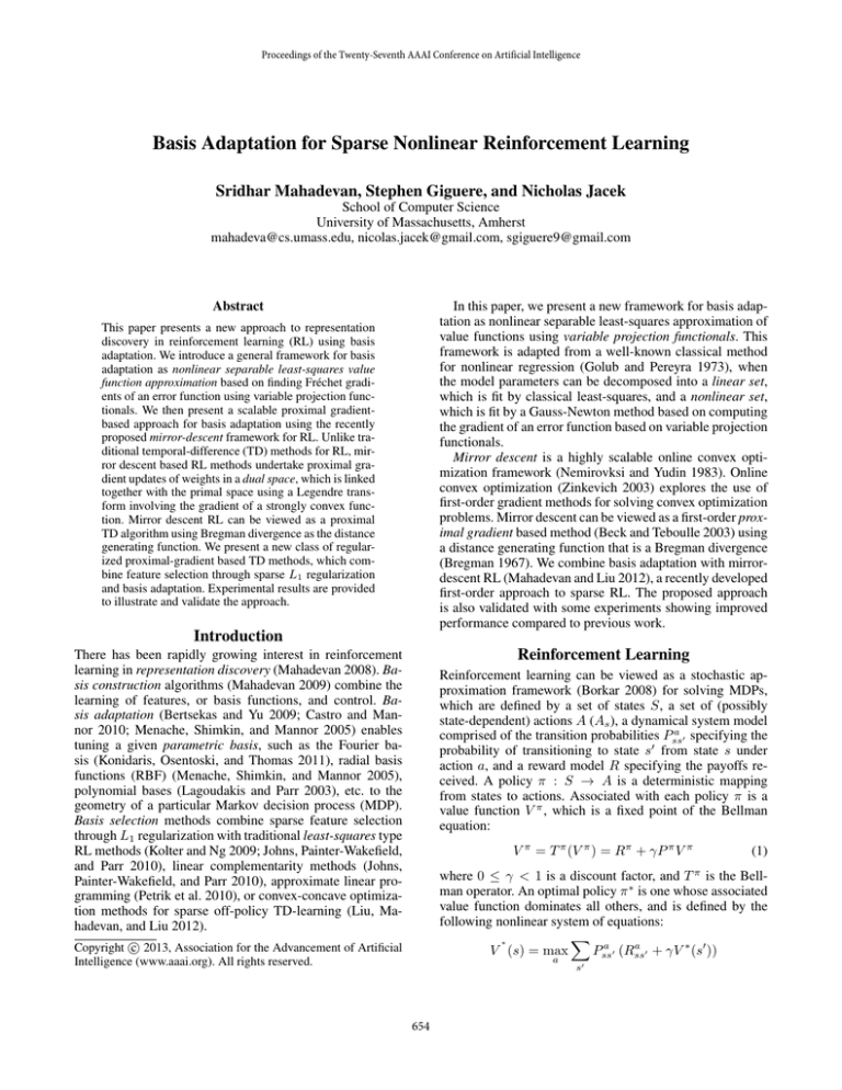
Figure 1: This figure shows the results of nonlinear basis
adaptation by solving the Bellman residual variable projection functional represented by Equation 8 to find the optimal
setting for the RBF centers and widths in a simple 25 state
chain domain. Top two figures: initial centers and widths of
RBF bases. Bottom two figures: Final centers and widths after convergence of nonlinear LSPI to the optimal policy.
α
α
problem involving the best selection of the nonlinear parameters α is computed by solving (a sampled version of)
Equation 8. We used lsqnonlin, a nonlinear least-squares
solver within MATLAB, to solve a sampled variant of Equation 8, where Φ(αt ) and P π Φ(αt ) were approximated by
their sampled counterparts Φ̂(αt ) and Φ̂ (αt ). Once α̂N BR
was found by the nonlinear phase, we used LSPI with these
settings to find the linear weights ŵN BR . Figure 1 illustrates
the application of this approach to a simple 25 state chain
domain (Lagoudakis and Parr 2003). The reward is at the
center, so the optimal policy is to go right in the first half
of the chain and go left otherwise. The Q function is approximated by a set of radial basis functions (RBFs), whose
initial centers and widths are specified as shown. The figure also shows the final modified centers and widths of the
RBFs using the Bellman residual variable projection functional minimization method.
We can rewrite the final result above as αN BR =
arg min Π⊥
Rπ 2 = arg min (I − Ψπα (Ψπα )† )Rπ 2 .
Ψπ
α
α
α
(8)
Given αN BR , the linear weights wN BR can be written as:
†
π
π
π
wN BR = Ψ⊥
Φ(αN BR ) R = ((I − γP )Φ(αN BR )) R
Comparing with Equation 6, the optimization problem for
nonlinear Bellman residual minimization once again involves minimization of a projector onto the complement of
a matrix column space, in this case Ψπα . We can state a new
result extending (Golub and Pereyra 1973) to the RL setting:
Theorem 2 Assume that Ψπα has constant rank r in every
open set Ω ⊂ Rk , where α ∈ Ω. If (αBR , wBR ) is the global
minimizer of Equation 7, then αN BR = αBR and wN BR =
wBR .
Nonlinear LSPI
Mirror Descent RL
We briefly describe a nonlinear variant of least-squares policy iteration (LSPI), where on each pass through the training data D = {st , at , rt , st+1 }, a nonlinear optimization
While the above framework of nonlinear separable value
function approximation using variable projection functionals is theoretically elegant, it can be computationally expensive to compute Fréchet gradients of the variable projection
functional in Equation 8 in large MDPs. We describe a novel
2
Similar VP functionals can be defined for other loss functions,
e.g. for the fixed point or TD case.
656
mirror-descent gradient-based approach to basis adaptation
that shows how to combine nonlinear value function approximation and sparsity.
Intuitively, the Bregman divergence measures the difference
between the value of a strongly convex function ψ(x) and
the estimate derived from the first-order Taylor series expansion at ψ(y). Many widely used distance measures turn
out to be special cases of Bregman divergences, such as
Euclidean distance (where ψ(x) =12 x22 ) and Kullback
Liebler divergence (where ψ(x) = i xi log2 xi , the negative entropy function). In general, Bregman divergences are
non-symmetric, but projections onto a convex set with respect to a Bregman divergence are well-defined.
The general mirror descent procedure can be written as:
1
wt+1 = argminw∈X w, ∂f (wt ) + Dψ (w, wt )
αt
(14)
Notice that the squared distance term in Equation 11 has
been generalized to a Bregman divergence. The solution to
this optimization problem can be stated succinctly as the following generalized gradient descent algorithm, which forms
the core procedure in mirror descent:
Proximal Mappings and Mirror Descent
Mirror descent can be viewed as a first-order proximal gradient method (Beck and Teboulle 2003; Zinkevich 2003)
for solving high-dimensional convex optimization problems.
The simplest online convex algorithm is based on the classic
gradient descent procedure for minimizing a convex function f , given as:
w0 ∈ X, wt = ΠX (wt−1 − βt ∇f (wt−1 )) : t ≥ 1
(9)
where ΠX (x) = argminy∈X x − y2 is the projector onto
set X, and βt is a stepsize. If f is not differentiable, then
the subgradient ∂f can be substituted instead, resulting in
the well-known projected subgradient method, a workhorse
of nonlinear programming (Bertsekas 1999) The proximal
mapping associated with a convex function h is defined as:
proxh (x) = argminu h(u) + u − x22
wt+1 = ∇ψ ∗ (∇ψ(wt ) − αt ∂f (wt ))
If h(x) = 0, then proxh (x) = x, the identity function.
If h(x) = IC (x), the indicator function for a convex set
C, then proxIC (x) = ΠC (x), the projector onto set C.
For learning sparse representations, the case when h(w) =
νw1 , for some scalar weighting factor ν, is particularly
important. In this case, the entry-wise proximal operator is:
⎧
⎨wi − ν, if wi > ν
(10)
proxh (w)i = 0,
if |wi | ≤ ν
⎩
wi + ν otherwise
Here, ψ ∗ is the Legendre transform of the strongly convex
function ψ, which is defined as
ψ ∗ (y) = sup (x, y − ψ(x))
x∈X
It can be shown that ∇ψ ∗ = (∇ψ)−1 (Beck and Teboulle
2003). Mirror descent is a powerful first-order optimization
method that been shown to be “universal” in that if a problem is online learnable, it leads to a low-regret solution using
mirror descent (Srebro, Sridharan, and Tewari 2011). It is
shown in (Ben-Tal, Margalit, and Nemirovski 2001) that the
mirror descent procedure specified in Equation 15 with the
Bregman divergence defined by the p-norm function (Gentile 2003), defined below, can outperform the projected subgradient method by a factor logn n where n is the dimensionality of the space. For high-dimensional spaces, this ratio
can be quite large.
An interesting observation follows from noting that the
projected subgradient method (Equation 9) can be written
equivalently using the proximal mapping as:
1
w − wt 22
wt+1 = argminw∈X w, ∂f (wt ) +
2βt
(11)
An intuitive way to understand this equation is to view the
first term as requiring the next iterate wt+1 to move in the
direction of the (sub) gradient of f at wt , whereas the second term requires that the next iterate wt+1 not move too far
away from the current iterate wt . Note that the (sub)gradient
descent is a special case of Equation (11) with Euclidean
distance metric. With this introduction, we can now introduce the main concept of mirror descent (Nemirovksi and
Yudin 1983). We follow the treatment in (Beck and Teboulle
2003) in presenting the mirror descent algorithm as a nonlinear proximal method based on a distance generating function
that is a Bregman divergence (Bregman 1967).
Definition 1: A distance generating function ψ(x) is defined as a continuously differentiable strongly convex function (with modulus σ) which satisfies:
x − x, ∇ψ(x ) − ∇ψ(x) ≥ σx − x2
Sparse Learning with Mirror Descent TD
Recently, a new framework for sparse regularized RL was
proposed based on mirror descent (Mahadevan and Liu
2012). Unlike regular TD, the weights are updated using the
TD error in the dual space by mapping the primal weights
w using a gradient of a strongly convex function ψ. Subsequently, the updated dual weights are converted back into the
primal space using the gradient of the Legendre transform of
ψ, namely ∇ψ ∗ . To achieve sparsity, the dual weights θ are
truncated according to Equation 10 to satisfy the l1 penalty
on the weights. Here, ν is the sparsity parameter. An analogous approach for l1 penalized classification and regression
was suggested in (Shalev-Shwartz and Tewari 2011).
One choice for Bregman divergence is the p-norm function, where ψ(w) = 12 w2q , and its conjugate Legendre
1
q q
transform ψ ∗ (w) = 12 w2p . Here, wq =
|w
|
,
j
j
(12)
Given such a function ψ, the Bregman divergence associated with it is defined as:
Dψ (x, y) = ψ(x) − ψ(y) − ∇ψ(y), x − y
(15)
and p and q are conjugate numbers such that p1 + 1q = 1. This
(13)
657
ψ(w) leads to the p-norm link function θ = f (w) where
f : Rd → Rd (Gentile 2003):
Algorithm 1 Mirror Descent Q(λ) with Basis Adaptation
1: Given: Parametric basis Φ(α)
2: Initialize linear parameters w0 and nonlinear parameters
α0 .
3: repeat
4:
Do action at = argmaxa∗ φt (st , a∗ ), wt with high
probability, else do a random action. Observe next
state st+1 and reward rt .
5:
Compute the actual TD error
sign(wj )|wj |q−1
sign(θj )|θj |p−1
, fj−1 (θ) =
q−2
wq
θp−2
p
(16)
Many other choices for Bregman divergence are possible.
fj (w) =
Basis Adaptation with Mirror Descent RL
Like the approach proposed for adaptive bases for Qlearning (Castro and Mannor 2010), our method is based
on the two-time scale stochastic approximation framework,
whereby the linear parameters w are adapted at a faster timescale than the nonlinear parameters α. Algorithm 1 below
describes the nonlinear adaptive basis mirror-descent variant
of Watkins Q(λ) algorithm.3 We indicate the dynamically
varying nature of the bases as φt (st , at ) where the subscript
denotes the particular value of the nonlinear parameters αt
at time t. In this section, we denote βt as the learning rate
for the faster time-scale update procedure for updating the
linear weights wt and ξt as the learning rate for the slower
time-scale parameter for updating the nonlinear basis parameters αt . Following the approach given in (Borkar 2008;
Castro and Mannor 2010), it can be shown that Algorithm 1
converges broadly under similar assumptions. The key idea
underlying Algorithm 1 is to adapt the nonlinear parameters
using the gradient of the TD error. As the gradient of the TD
error is not easily computed due to the max computation
in Q(λ), what is done here is to approximate the maximum
using a smoothed differentiable approximation (Castro and
Mannor 2010):
max xi ≈ fσ ({xi }i=1,...,n ) = log(
i=1,...,n
n
δt = rt + γ maxφt (st+1 , a), wt − φt (st , at ), wt a
6:
Compute the smoothed TD error
ωt = rt +γfσ ({φt (st+1 , a ), wt }a )−φt (st , at ), wt 7:
Compute the gradient of the smoothed TD error w.r.t..
α
∂fσ ({φt (st+1 , a ), wt }a )
Kσ (st , at , st+1 ) = γ
∂(φt (st+1 , a ), wt )
a
× ∇α (φt (st+1 , a ), wt ) − ∇α (φt (st+1 , at ), wt )
8:
9:
10:
Update the eligibility trace et ← et + λγφt (st , at )
Update the dual weights θt = ∇ψt (wt )+βt δt et (e.g.,
ψ(w) = 12 w2q is the p-norm link function).
Truncate weights:
∀j, θjt+1 = sign(θ̃jt+1 ) max(0, |θ̃jt+1 | − βt ν)
11:
12:
eσxi )
Update linear weight parameters: wt+1
=
∇ψt∗ (θt+1 ) (e.g., ψ ∗ (θ) = 12 θ2p and p and q
are dual norms such that p1 + 1q = 1).
Update nonlinear basis parameters:
αt+1 ← αt + ξt ωt Kσ
i=1
13:
Set t ← t + 1.
14: until done.
We update the nonlinear basis parameters αt on a slower
time scale using the gradient of the smoothed TD error. The
mirror-descent version of Watkins Q(λ) with basis adaptation is given below.
Return Q̂(s, a) = (Φ(αt )wt )s,a as the approximate l1
penalized sparse optimal action value function.
Experimental Results
In this section, we provide some illustrative experiments
evaluating the performance of the mirror-descent Q(λ)
method with a nonlinear generalization of the fixed Fourier
basis (Konidaris, Osentoski, and Thomas 2011). The nonlinear Fourier basis that we used is as follows:
can be seen here as a weighting of how important each ci is.
In our initial experiments, we vary both α and ci separately
to compare their effects.
Figure 2 compares the convergence and stability of Q(λ)
and mirror-descent Q(λ) using 49 fixed Fourier bases with
mirror-descent Q(λ) using the same number of adaptive (α
and Ci parameter tuned) nonlinear Fourier bases. In this
case, all methods converge, but the two nonlinear mirrordescent methods (bottom curves) converge much more
quickly. The mirror-descent methods have converged by 7
episodes to an average solution length at least thrice as small
as the regular Q(λ) method, which takes much longer to
reliably achieve the same solution quality. For the experimental result shown in Figure 2, where we show convergence in the mountain car domain with 49 Fourier bases,
we set βt = 0.03, ξt = 5 × 10−7 , and ν = 0.001.
The p-norm Bregman divergence was used, where p =
φi (x) = cos(παi ci , x)
The nonlinear parameters here include both αi and ci . Note
that in the previous work on Fourier bases (Konidaris, Osentoski, and Thomas 2011), the scaling factor αi was fixed
to unity, whereas in our case, it is allowed to vary (as shown
in Figure 4). Also, earlier work set ci = [c1 , . . . , cd ], cj ∈
[0, . . . , n], 1 ≤ j ≤ d. For example, in the mountain car domain, d = 2, and setting n = 3 would result in 16 possible
features (since n = 0, 1, 2, 3). The nonlinear parameter αi
3
The extension to related methods like SARSA(λ) (Sutton and
Barto 1998) is straightforward. Some details abbreviated for clarity.
658
showing they not only result in improved performance, but
also lower variance. Finally, Figure 4 shows the ranges of
the α parameters as tuned by the basis adaptation algorithm
for 49 Fourier bases over 25 runs.
Comparison of Four Methods over 25 runs
500
450
350
Mirror Descent Q(lambda) with Nonlinear Fourier Basis: 25 runs
1100
300
1000
250
200
150
Q(λ)
Mirror−Descent Q(λ)
100
Nonlinear Mirror−Descent Q(λ) α
50
Nonlinear Mirror−Descent Q(λ) Ci
0
0
2
4
6
8
10
900
steps to completion
steps to completion
400
12
14
16
18
800
700
600
500
400
300
200
20
episode number (features = 49, learn rate: 0.03)
100
0
0
5
10
15
20
25
30
35
40
45
episode number (features = 49, learn rate: 0.03)
Figure 2: Comparing the convergence of two mirror-descent
Q(λ) methods over 25 runs with 49 (α and ci parameter
tuned) nonlinear Fourier bases in the mountain car task with
that of Q(λ), and mirror-descent Q(λ), with 49 fixed Fourier
bases.
Mirror Descent Q(Lambda) With Nonlinear Fourier Basis Weights: 25 runs
Fourier Basis Scale
1.15
2 log10 (num features x num actions), and q =
The
learning rate for Q(λ) had to be set fairly low at 0.001 when
the number of features exceeded 16 as higher rates caused
instability.
p
p−1 .
1.1
1.05
1
0.95
0.9
400
300
200
100
0
0
5
10
15
20
episode number (learn rate: 0.03)
500
400
200
100
0
0
300
200
100
0
0
5
10
15
20
episode number (learn rate: 0.03)
5
10
15
20
episode number (learn rate: 0.03)
Conclusions and Future Work
Q(lambda): 25 runs
steps to completion
steps to completion
400
Figure 4: (a) Extended run of the mirror-descent Q(λ)
method with basis adaptation of the α parameters in the
mountain car domain. (b) Boxplot of the α parameters for
49 Fourier bases for the run shown on top.
300
Mirror Descent Q(lambda): 25 runs
500
Fourier Basis Parameter (features = 49, learning rate: 0.03)
Mirror Descent Q , Nonlinear Alpha
steps to completion
steps to completion
Mirror Descent Q Nonlinear Ci
500
500
This paper introduced a broad framework for basis adaptation as nonlinear separable least-squares value approximation, and described a specific gradient-based method for basis adaptation using mirror descent optimization. Currently,
the learning rate for nonlinear parameters needs to be set
quite low for stable convergence. More rapid tuning of the
nonlinear parameters could be achieved by including an additional mirror descent step for modifying them.
400
300
200
100
0
0
5
10
15
20
episode number (learn rate: 0.001)
Acknowledgments
Figure 3: Variance of the four methods compared in Figure 2
across 25 runs. Note the improved variance of the two methods shown on top that combine mirror-descent updating and
basis adaptation.
This research is supported in part by the Air Force Office
of Scientific Research (AFOSR) under grant FA9550-101-0383, and the National Science Foundation under Grant
Nos. NSF CCF-1025120, IIS-0534999, IIS-0803288, and
IIS-1216467 Any opinions, findings, and conclusions or recommendations expressed in this material are those of the author and do not necessarily reflect the views of the AFOSR
or the NSF.
Figure 3 shows the variance across 25 runs of the four
methods compared in Figure 2. Note the improved variance
of the two mirror-descent methods that use basis adaptation,
659
References
Mahadevan, S. 2008. Representation Discovery using Harmonic Analysis. Morgan and Claypool Publishers.
Mahadevan, S. 2009. Learning Representation and Control
in Markov Decision Processes: New Frontiers. Foundations
and Trends in Machine Learning 1(4):403–565.
Menache, N.; Shimkin, N.; and Mannor, S. 2005. Basis function adaptation in temporal difference reinforcement
learning. Annals of Operations Research 134:215–238.
Nemirovksi, A., and Yudin, D. 1983. Problem Complexity
and Method Efficiency in Optimization. John Wiley Press.
Petrik, M.; Taylor, G.; Parr, R.; and Zilberstein, S. 2010.
Feature selection using regularization in approximate linear
programs for markov decision processes. In ICML, 871–
878.
Shalev-Shwartz, S., and Tewari, A. 2011. Stochastic methods for l1 regularized loss minimization. Journal of Machine
Learning Research.
Srebro, N.; Sridharan, K.; and Tewari, A. 2011. On
the universality of online mirror descent. Arxiv preprint
arXiv:1107.4080.
Sutton, R., and Barto, A. G. 1998. An Introduction to Reinforcement Learning. MIT Press.
Watkins, C. 1989. Learning from Delayed Rewards. Ph.D.
Dissertation, King’s College, Cambridge, England.
Zinkevich, M. 2003. Online convex programming and generalized infinitesimal gradient ascent. Proceedings of the
International Conference on Machine Learning (ICML).
Beck, A., and Teboulle, M. 2003. Mirror descent and nonlinear projected subgradient methods for convex optimization.
Operations Research Letters.
Ben-Tal, A.; Margalit, T.; and Nemirovski, A. 2001. The ordered subsets mirror descent optimization method with applications to tomography. SIAM Journal of Optimization.
Bertsekas, D. P., and Tsitsiklis, J. N. 1996. Neuro-Dynamic
Programming. Belmont, Massachusetts: Athena Scientific.
Bertsekas, D., and Yu, H. 2009. Basis function adaptation
methods for cost approximation in Markov Decision Processes. In IEEE International Symposium on Adaptive Dynamic Programming and Reinforcement Learning.
Bertsekas, D. P. 1999. Nonlinear Programming. Athena
Scientific, 2nd edition.
Borkar, V. 2008. Stochastic Approximation: A Dynamical
Systems Viewpoint. Cambridge University Press.
Bregman, L. 1967. The relaxation method of finding the
common point of convex sets and its application to the solution of problems in convex programming. USSR Computational Mathematics and Mathematical Physics 7(3):200 –
217.
Castro, D. D., and Mannor, S. 2010. Adaptive bases for Qlearning. In 49th IEEE Conference on Decision and Control.
Geist, M., and Scherrer, B. 2011. L1-penalized projected
Bellman residual. In Proceedings of the European Workshop
on Reinforcement Learning.
Gentile, C. 2003. The robustness of the p-norm algorithms.
Mach. Learn. 53:265–299.
Golub, G., and Pereyra, V. 1973. The differentiation of
pseudo-inverses and nonlinear least squares problems whose
variables separate. SIAM Journal of Numerical Analysis
10:413–32.
Johns, J.; Painter-Wakefield, C.; and Parr, R. 2010. Linear complementarity for regularized policy evaluation and
improvement. In Proceedings of Advances in Neural Information Processing Systems 23.
Kolter, J. Z., and Ng, A. Y. 2009. Regularization and feature
selection in least-squares temporal difference learning. In
Proceedings of the 26th Annual International Conference on
Machine Learning, ICML ’09, 521–528. New York, NY,
USA: ACM.
Konidaris, G.; Osentoski, S.; and Thomas, P. 2011. Value
function approximation in reinforcement learning using the
fourier basis. In Proceedings of the Twenty-Fifth Conference
on Artificial Intelligence.
Lagoudakis, M., and Parr, R. 2003. Least-squares policy
iteration. Journal of Machine Learning Research 4:1107–
1149.
Liu, B.; Mahadevan, S.; and Liu, J. 2012. Regularized offpolicy TD-learning. In Neural Information Processing Systems Conference (NIPS).
Mahadevan, S., and Liu, B. 2012. Reinforcement learning
using mirror descent. In UAI 2012: Proceedings of the conference on Uncertainty in AI.
660