Proceedings of the Twenty-Eighth AAAI Conference on Artificial Intelligence
Avoiding Plagiarism in Markov Sequence Generation
Alexandre Papadopoulos, 1,2 Pierre Roy, 1 François Pachet1,2
1
2
Sony CSL, 6 rue Amyot, 75005, Paris, France
Sorbonne Universités, UPMC Univ Paris 06, UMR 7606, LIP6, F-75005, Paris, France
Abstract
Markov processes are widely used to generate sequences that imitate a given style, using random walk.
Random walk generates sequences by iteratively concatenating states to prefixes of length equal or less than
the given Markov order. However, at higher orders,
Markov chains tend to replicate chunks of the corpus
with a size possibly higher than the order, a primary
form of plagiarism. The Markov order defines a maximum length for training but not for generation. In the
framework of constraint satisfaction (CSP), we introduce M AX O RDER. This global constraint ensures that
generated sequences do not include chunks larger than
a given maximum order. We exhibit an automaton that
recognises the solution set, with a size linear in the size
of the corpus. We propose a linear-time procedure to
generate this automaton from a corpus and a given max
order. We then use this automaton to achieve generalised arc consistency for the M AX O RDER constraint,
holding on a sequence of size n, in O(n.T ) time, where
T is the size of the automaton. We illustrate our approach by generating text sequences from text corpora
with a maximum order guarantee, effectively controlling plagiarism.
p(si+1 |s1 , . . . , si ) = p(si+1 |si−k+1 , . . . , si ).
In theory, higher order Markov models are equivalent to
order 1 models. However, in practice, higher order models
offer a better compromise between expressivity and representation cost. Variable order Markov models are often used
to produce sequences with varying degrees of similarity with
the corpus (Begleiter, El-Yaniv, and Yona 2004). Indeed, increasing the Markov order produces sequences that replicate
larger chunks of the original corpus, thereby improving the
impression of style imitation.
However, it has also been long observed (Brooks et al.
1957) that increasing the order tends to produce sequences
that contain chunks of the corpus of size much larger than
the Markov order.
We illustrate this phenomenon on a text corpus: Johnston’s English translation of Pushkins Eugene Onegin – a
reference to Markov, as he used the same corpus (in Russian)
for his pioneering studies. Here, an element of the Markov
chain is a word of the text or a sentence separator, and a
sequence is a succession of such elements. With a Markov
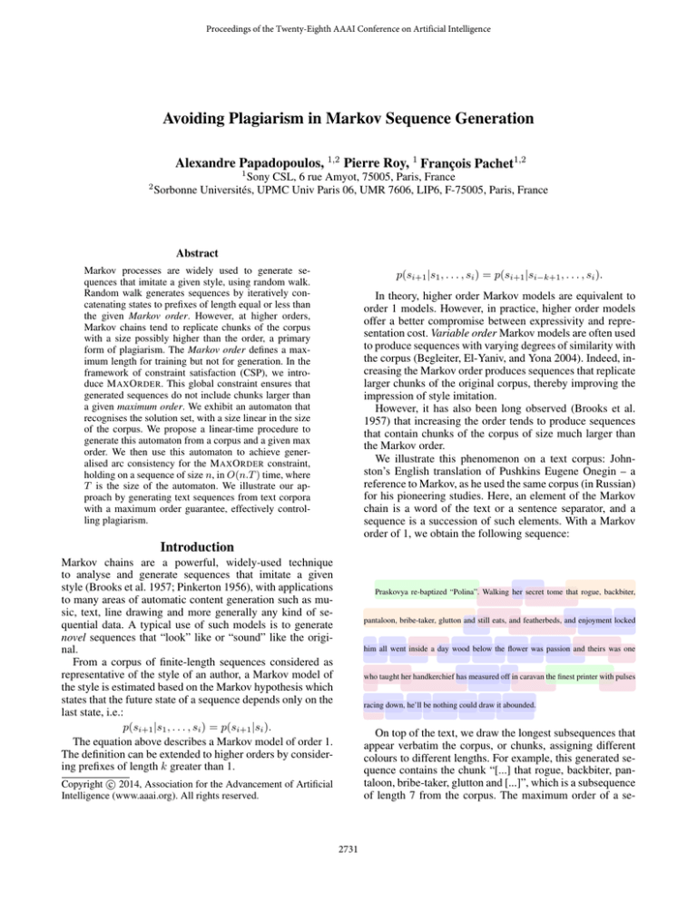
order of 1, we obtain the following sequence:
Introduction
Markov chains are a powerful, widely-used technique
to analyse and generate sequences that imitate a given
style (Brooks et al. 1957; Pinkerton 1956), with applications
to many areas of automatic content generation such as music, text, line drawing and more generally any kind of sequential data. A typical use of such models is to generate
novel sequences that “look” like or “sound” like the original.
From a corpus of finite-length sequences considered as
representative of the style of an author, a Markov model of
the style is estimated based on the Markov hypothesis which
states that the future state of a sequence depends only on the
last state, i.e.:
p(si+1 |s1 , . . . , si ) = p(si+1 |si ).
The equation above describes a Markov model of order 1.
The definition can be extended to higher orders by considering prefixes of length k greater than 1.
Praskovya re-baptized “Polina”. Walking her secret tome that rogue, backbiter,
pantaloon, bribe-taker, glutton and still eats, and featherbeds, and enjoyment locked
him all went inside a day wood below the flower was passion and theirs was one
who taught her handkerchief has measured off in caravan the finest printer with pulses
racing down, he’ll be nothing could draw it abounded.
On top of the text, we draw the longest subsequences that
appear verbatim the corpus, or chunks, assigning different
colours to different lengths. For example, this generated sequence contains the chunk “[...] that rogue, backbiter, pantaloon, bribe-taker, glutton and [...]”, which is a subsequence
of length 7 from the corpus. The maximum order of a se-
c 2014, Association for the Advancement of Artificial
Copyright Intelligence (www.aaai.org). All rights reserved.
2731
Markov order
1
2
3
4
5
6
median
2
2
9
45
78
78
lower quartile
2.0
2.0
6.0
28.0
77.0
78.0
upper quartile
3.0
3.0
13.0
65.0
79.0
79.0
of the sequence to generate. Markov constraints enforce that
variables in the sequence should have valid Markov continuations. Sequence generation is obtained by CSP resolution.
Additional constraints can be easily introduced to control the
generation of the sequence. In practice, the problem boils
down to the identification of efficient arc-consistency algorithms for the given constraints.
Under this framework, we introduce the M AX O RDER
global constraint. It holds on all the variables of the CSP,
and states that 1) the sequence is a valid order k Markov
sequence, and 2) no L consecutive variables form a sequence that belongs to the training corpus. Following Pesant (2004) and Beldiceanu, Carlsson, and Petit (2004), we
enforce generalised arc-consistency by feeding a constraint
such as R EGULAR an automaton that accepts the set of such
sequences. However, we show that canonical methods are
not satisfactory for building this automaton. The main contribution of this paper is a linear-time algorithm that builds
this automaton.
Table 1: Maximum orders for different Markov orders
quence is the maximum length of its chunks (7, in our example).
If we increase the order to 3, we obtain sequences such as
the following one:
Love’s frantic torments went on beating and racking with their strain and stress that
youthful heart. It all seemed new – for two days only – the estate provides a setting
Running Example
for angry heirs, as one, to admire him – and replies: Wait, I’ll present you – but inside
We consider the corpus made of ABRACADABRA, where
each element is one of the symbols A, B, C, D or R. With
k = 1, the Markov chain estimated on this corpus is given
by the following transition matrix:
a day, with custom, love would fade away. It’s right and proper that you transcend in
music’s own bewitching fashion the foreign words a maiden’s passion found for its
A
B
C
D
R
utterance that night directed his.
This sequence makes arguably more sense than the one
generated with order 1. However, its maximum order is 20
(i.e. it contains a 20-word-long subsequence copied verbatim from the corpus). To any reader familiar with the corpus,
this would read like blatant plagiarism.
To illustrate this phenomenon in a more general way, we
generated a few hundreds of sequences of varying order
(from to 1 to 6). Table 1 shows the maximum order observed
for each Markov order: this value increases to values much
higher than the Markov order. Markov order affects training: when estimated from a corpus, the Markov model learns
all continuations of sequences of k states or less. However,
this parameter k does not limit the maximum order of the
generated sequence. In particular, the whole corpus itself is
trivially a valid Markov sequence of order k.
This paper addresses precisely the problem of generating
Markov sequences with an imposed maximum order. Such
sequences cannot be obtained with greedy approaches like
random walk. However, the maximum order problem can be
seen as a specific instance of a constrained Markov problem. Introduced by Pachet and Roy (2011), Markov constraints consist in reformulating the generation of Markov
sequences as a combinatorial problem (CSP). By enforcing arc-consistency of the Markov constraints, we can solve
such a CSP in a backtrack-free manner, thus simulating a
greedy random walk generation procedure.
As opposed to greedy approaches, the Markov constraint
approach guarantees a complete exploration of the space of
sequences. The variables of this CSP represent the elements
A
0
0
1

1
1
B
0.5
0
0
0
0
C
0.25
0
0
0
0
D
0.25
0
0
0
0
R
0
1
0

0
0
During a training phase, these probabilities are estimated
according to their frequency in the corpus. Here, in the four
continuations for A in the corpus, two are with B, one with
C and one with D. A sequence is a Markov sequence, according to an order k Markov chain, if every k-gram of the
sequence has a continuation with a non-zero probability. For
example, ABRADABRACA is a valid Markov sequence,
but ABRACADABA is not a valid Markov sequence, because the probability of having A after B is zero.
Automaton Representation
Following the works on language automata and global constraints, we can encode a set of Markovian sequences using an automaton. Global constraints such as R EGULAR can
then take this automaton as input to generate sequences.
Definition 1 (Automata). A deterministic finite-state automaton, or, simply, automaton, is a quintuple A =
hQ, Σ, δ, q0 , F i, where:
•
•
•
•
Q is a finite non-empty set of states;
Σ is the alphabet – a finite non-empty set of symbols;
q0 ∈ Q is the initial state of the automaton;
δ is the transition function Q × Σ → Q, which maps a
state to its successors for a given symbol;
• F ⊆ Q is the set of final, or accepting, states.
2732
B
B
R
R
C
A
D
R
R
B
B
A
C
D
A
C
D
D
C
A
A
Figure 1: A Markov automaton for the ABRACADABRA
corpus, with k = 1
RA
BR
C
A
RAC
Definition 2 (Accepted language). An automaton recognises, or accepts, a set of words, called a language, defined
as follows.
• A word w ∈ Σ∗ is a sequence a1 . . . ap of symbols ai ∈
Σ.
• The word w is accepted by A if and only if there exists a
sequences q0 , . . . , qp of states, such that δ(qi−1 , ai ) = qi ,
for all i, 1 ≤ i ≤ p, and qp ∈ F .
• L(A) = {w ∈ Σ∗ |w is accepted by A} is the accepted
language of A.
In order to represent order k Markov transitions, we create
an alphabet Σ where each symbol corresponds to a unique kgram of the corpus. Then, a valid order k Markov transition
is represented by two symbols, such that their two corresponding k-grams overlap on their common k − 1 symbols.
A valid Markov sequence of length n is represented by a
word of length n − k + 1 on this alphabet.
For example, for k = 2, the sequence ABRA corresponds
to a sequence of three 2-grams hA, Bi, hB, Ri, hR, Ai. We
can assign three symbols a1 , a2 , a3 ∈ Σ to those three
2-grams in their respective order. The Markov transition
A, B → R is represented by the word a1 a2 , and the sequence ABRA by the word a1 a2 a3 .
Definition 3 (Markov Automaton). A Markov automaton
associated to a corpus is an automaton A such that L(A) =
{a1 . . . an ∈ Σ∗ |ai ai+1 is a Markov transition, ∀i, 1 ≤ i ≤
n}
Figure 1 shows a Markov automaton for the corpus
ABRACADABRA with k = 1.
We can now represent the set of Markov sequences satisfying the maximum order property as the following automaton.
Definition 4 (Maximum Order Automaton). Let M be a
Markov automaton for a given corpus. For a given no-good
a1 . . . aL ∈ N , let A(a1 . . . aL ) be an automaton such that
L(A(a1 . . . aL )) = {w ∈ Σ∗ |a1 . . . aL is a factor of w}, i.e.
the language of words containing at least one occurrence of
the no-good. An automaton MO is a maximum order automaton for C and N if:
\
L(MO) = L(M) ∩
L(A(a1 . . . aL ))
RD B
BRA
B
AB
R
ABR
BB
D
B
AD
AD D
ADA
C
D
C
AC
C
C
A
ACA
A
A
CA
DA
D
B
CAD
DAB
C
Figure 2: A maximum order automaton for the ABRACADABRA corpus, with k = 1 and L = 4
The M AX O RDER Constraint
The purpose of M AX O RDER is to generate Markov sequences with a guaranteed maximum order. The constraint
takes two parameters C and N ; C ⊆ Σ2 denotes a set of
valid Markov transitions, each represented by an element
a1 a2 ∈ C corresponding to a valid pair of k-grams; N ⊆ ΣL
denotes a set of forbidden sequences, or no-goods.
In practice, each no-good of size L = L0 − k + 1 corresponds to a sequence of size L0 that appears in the corpus,
where k is the Markov order, and L0 is the maximum order.
M AX O RDER is defined as follows.
Definition 5 (M AX O RDER constraint). The constraint
M AX O RDER(C, N , X1 , . . . , Xn ) holds iff:
• for each i, 1 ≤ i < n, Xi Xi+1 ∈ C;
• for each i, 1 ≤ i < n − L0 + 1, Xi . . . Xi+L0 −1 6∈ N .
For example consider the ABRACADABRA corpus, with
k = 1 and L = 4. There are 7 no-goods: ABRA,
BRAC, RACA, ACAD, CADA, ADAB, DABR. The Markovian sequence ABRADABRACA does not satisfy the maximum order property: it contains the no-goods ABRA,
ADAB, DABR, BRAC, RACA. The Markovian sequence
RADADACAB does not contain any no-good of size 4, and
so satisfies the maximum order property for L = 4. In fact,
any satisfying sequence is a substring of a string following
the pattern BRA(DA)+ (CA)+ BR.
Propagating the M AX O RDER Constraint
There is a canonical way to propagate M AX O RDER by considering the maximum order automaton. Then, we can enforce the M AX O RDER constraint by imposing a sequence of
variables to form a word recognised by this automaton, using the R EGULAR constraint (Pesant 2004). If T is the size
of the automaton (the number of transitions), generalised
arc-consistency on a sequence of n variables is achieved in
O(n.T ) time.
The maximum order automaton can be built using standard automata theory operations that implement Definition 4. Initially, we build a Markov automaton (we provide
a1 ...aL ∈N
Figure 2 shows a maximum order automaton for the corpus ABRACADABRA, with k = 1 and L = 4. The labels
in the states correspond to prefixes of forbidden no-goods.
2733
in this paper an algorithm for doing this). Then, for each nogood, this automaton is intersected with the negation of the
automaton recognising sequences containing the no-good.
However, the complexity of this procedure is dominated
by the complexity of intersecting a number of automata. If
O(t) is the size of any of the automata, and N = |N | is the
number of no-goods, the complexity is O(tN ). It is unlikely
that an algorithm with a better complexity exist (Karakostas,
Lipton, and Viglas 2000; 2003). Furthermore, this method
does not give any bound on the size of the final automaton
(other than O(tN )). In the following section, we propose a
linear-time algorithm to build this automaton.
Algorithm 1: Markov automaton
Data: C the set of valid Markovian transitions
Result: M the minimal Markov automaton
1
2
3
4
5
6
7
8
9
Algorithms
10
In this section, we build the maximum order automaton in
time linear in the size of the input, the set of no-goods. As a
corollary, we show that the size T of this automaton is linear in the size of the input, and, therefore, that propagating
the M AX O RDER is polynomial too. To this end, we introduce two algorithms. The first algorithm builds the minimal
Markov automaton. The second algorithm builds a trie with
the no-goods, computes their overlaps, and uses it to remove
from the Markov automaton all sequences containing a nogood.
11
12
13
14
15
16
17
18
19
20
Markov automaton
21
The first algorithm consists in building an automaton recognising all Markovian sequences, i.e. sequences where any
two successive k-grams correspond to a k + 1-gram of the
corpus, for a Markov order of k. This automaton, when
viewed as a labelled directed graph, is essentially a syntactic
rewrite of the Markov chain, with a different semantics attached to its nodes and edges. In this automaton, each transition is labelled by a symbol corresponding to a Markov
state. A notable property of a Markov automaton is that all
transitions labelled with a given symbol point to the same
state.
22
23
M ← hQ, Σ, δ, q0 , F i
q ← NewState(Q)
a(q) ← ∅
forall the a ∈ Σ do
δ(q0 , a) ← q
Q(a) ← q; a(q) ← a(q) ∪ {a}
F ← F ∪ {q0 , q}
forall the a1 a2 ∈ C do
q1 ← Q(a1 )
q ← separate(q1 , a1 )
q2 ← Q(a2 )
δ(q, a2 ) ← q2
if ∃q 0 ∈ Q such that q and q 0 are equivalent then
Merge q with q 0
Q(a1 ) ← q 0 ; a(q 0 ) ← a(q 0 ) ∪ a(q)
function separate(q1 , a1 )
q ← NewState(A)
accept(q) ← True
forall the a ∈ Σ such that δ(q1 , a) is def do
δ(q, a) ← δ(q1 , a)
forall the q 0 ∈ Q such that δ(q 0 , a1 ) = q1 do
δ(q 0 , a1 ) ← q
Q(a1 ) ← q; a(q) ← {a1 }
all ingoing a1 -labelled transitions from q1 to the newly created state. An a2 -labelled transition can be added. Minimality is incrementally maintained by assuming the invariant
that, before the call to separate(), all states are pairwise non-equivalent. The creation of q does not affect the
equivalency of any other state (in particular, not the predecessors of q and q1 ). After we add an a2 -labelled transition
to q, q ceases to be equivalent with q1 . However, with the
addition of the transition, it might have become equivalent
to a (unique) other state, in which case we merge them, thus
maintaining the invariant.
The size of the resulting automaton and the running time
to build it, are both bounded by the number of transitions in
C.
Definition 6 (State labels). We use the following notation
to relate states and the labels of its ingoing transitions.
• Let q be a state, a(q) = {a ∈ Σ|∃q 0 ∈ Q, δ(q 0 , a) = q} is
the set of labels of the transitions pointing to q.
• Let a be a symbol of the alphabet, Q(a) is the unique state
q such that a ∈ a(q).
The interpretation of a Markov automaton A can be stated
formally as follows. Let a1 , a2 ∈ Σ be two symbols. A
Markov transition between the k-grams corresponding to a1
and a2 is represented in A by a transition between Q(a1 ) and
Q(a2 ), labelled by a2 . Intuitively, when at state q = Q(a1 ),
we can observe any one of the Markov states in a(q). If we
observe a1 , we can generate a2 . Since the automaton accepts
sequences of arbitrary length, all states are accepting.
We build the Markov automaton using Algorithm 1. First
a state is created that observes any Markov state (Lines 2
to 7). Then, each Markov transition is inserted iteratively.
When inserting (a1 , a2 ), a new state q is created using the
separate() function. This function creates a new state,
which has the same outgoing transitions as q1 , and redirects
Maximum Order Automaton
The second algorithm consists in removing from the Markov
automaton any sequence that contains at least one no-good,
i.e. a sequence of forbidden length appearing in the corpus.
This is performed by Algorithm 2. Intuitively, a trie of the
no-goods is computed, where all states but the ones corresponding to a full no-good are accepting states. This ensures
that a no-good is never accepted. However, this is not sufficient. The key part of the algorithm is to add the connection
between overlapping prefixes. For example, if we have two
no-goods ABCD and BCEF, the prefixes ABC and BCEF
2734
In more details, this algorithm first disconnects from
the Markov automaton any transition that starts a no-good.
Then, those transitions are extended to a full trie of all the
no-goods. For a state q of the trie, w(q) records the prefix recognised by this state, i.e. the word accepted from q0
to q. By excluding the states that recognise a complete nogood (line 20), we guarantee that no sequence including any
no-good will be recognised. However, we are not removing
those states yet. We first have to deal with a key aspect of this
algorithm, which concerns the overlap between no-goods.
For example, with two no-goods ABCD and BCEF, supposing we started ABC, we cannot continue with D, as this
would complete a no-good. However, if we continue with E,
we start the no-good BCEF. Therefore, a cross-prefix transition between the state for ABC and the state for BCE must
be added. Cross-prefix transitions ensure that, by avoiding a
particular no-good, we will not inadvertently complete another no-good. We use an adaptation of the Aho and Corasick string-matching algorithm (Aho and Corasick 1975):
when we use a transition that does not extend the current
prefix, we can jump directly to the longest no-good that is
a suffix of the current prefix. Finally, we add transitions in
the trie for any state missing some valid Markov transitions.
Those transitions either point back to the original Markov
automaton, for Markov transitions that do not start any nogood, or point to the states of the first layer of the trie, for
Markov transitions that start a new no-good. Since we kept
the transitions to the non-accepting states that complete a nogood, we know we are not introducing any no-good. We can
know finally remove those non-accepting states (line 34).
The algorithm adds exactly once each transition of the resulting automaton. Therefore, it runs in time linear in the
number T of transitions of the final automaton. Let N =
L.|N | be size of the input N . When constructing the trie,
it creates exactly N transitions. During the next phase, the
added transitions are exactly those added by the Aho and
Corasick algorithm. Their number is linearly bounded by N ,
a (non-trivial) result from Aho and Corasick (1975). Finally,
the number of transitions added to each state during the completion phase is bounded by |Σ|, which is independent of N .
Note that the general idea of this algorithm is similar to
the algorithm by (Villeneuve and Desaulniers 2005), which
computes shortest paths with forbidden paths. However, they
operate in a very different context, and are only interested in
shortest paths, whereas we are interested in all sequences.
Algorithm 2: M AX O RDER AUTOMATON
Data: N the set of forbidden no-goods
M ← hQ, Σ, δ, q0 , F i: a Markov automaton
Result: Any word containing at least one no-good is not
recognised by M
1
2
3
4
5
6
7
8
9
10
11
12
13
14
15
16
17
18
19
20
21
22
23
24
25
26
27
// Remove transitions that start a
no-good
forall the a1 . . . aL ∈ N do
q ← Q(a1 )
q ← separate(q, a1 )
Clear outgoing transitions of q
w(q) ← (a1 )
// Compute the trie of no-goods
Qtrie ← ∅
forall the a1 . . . aL ∈ N do
q ← q0
i←1
while δ(q, ai ) exists do
q ← δ(q, ai )
i←i+1
for aj , i ≤ j ≤ L do
q 0 ← NewState(Qtrie )
F ← F ∪ {q 0 }
δ(q, aj ) ← q 0
w(q 0 ) ← (a1 , . . . , aj )
a(q 0 ) ← {aj }
q ← q0
F ← F \ {q}
// Compute cross prefix transitions
forall the q ∈ Qtrie do
S(q) ← {q 0 ∈ Qtrie |w(q)is a strict suffix of w(q 0 )}
forall the q ∈ Qtrie in order of decreasing |w(q)| do
forall the a ∈ Σ such that δ(q, a) exists do
forall the q 0 ∈ S(q) do
if δ(q 0 , a) is undefined then
δ(q 0 , a) ← δ(q, a) // transition
is Markovian
28
33
// Markovian completion
forall the ∀q ∈ Qtrie do
{a1 } ← a(q)
forall the a2 ∈ Σ such that a1 a2 ∈ C do
if δ(q, a2 ) is undefined then
δ(q, a2 ) ← Q(a2 )
34
Q ← Q ∪ (Qtrie ∩ F )
29
30
31
32
Generating Sequences with a Maximum Order
guarantee
We can use the maximum order automaton to generate sequences, by using any implementation of R EGULAR. In
practice, we use a decomposition based method (Quimper
and Walsh 2006; 2008), which works better in practice with
large automata, by exploiting efficient propagators for extensional (table) constraints.
In order to simulate a random walk procedure with a variable order, we chose the following variable and value ordering heuristics. We use static variable ordering heuristics, in
their temporal order. For a given variable Xi , we consider
up to k previous variables. We then consider all the contin-
overlap on BC. This means that the automaton should not
accept ABCD, but it should not accept ABCEF either. This
connection is made using cross-prefix transitions. In order to
achieve this, Algorithm 2 uses an adaptation of the Aho and
Corasick (1975) string-matching algorithm.
2735
solution loss
1
“
0.8
0.6
0.4
0.2
0
6 8 10 12 14 16 18 20
L
Figure 3: Solution loss from M AX O RDER, on “Eugene Onegin” with k = 3, n = 20, for various values of L
uations in the corpus for the sequence Xi−k , . . . , Xi−1 that
are arc-consistent for M AX O RDER. If the number of such
continuations is above a certain fixed threshold, we choose
one, using the transition probabilities. Otherwise, the procedure is repeated for a smaller k, until one value is found.
We start with k = L − 1. Note that using the transition
probabilities does not necessarily generate sequences with
the right probability distribution (Pachet, Roy, and Barbieri
2011). This is however a reasonable approximation in the
context of this paper.
A resolution on this model will be backtrack-free, and
will simulate a random walk with a variable order – with the
aforementioned caveat concerning transition probabilities –
with the maximum order guarantee.
Blessed is he who’s left the squire no time devoted to the North.
After that, you’re married: no look, no word to say and then began
to lift his pistol in his glance, or else. The friends in all that is the
one. Ah Tanya, come to know it in the fashion and in second all
in fever. We must confess that all of an earlier time. Look to the
circle of our first ages from thirty down to the end. He’s moved.
For cousins from afar, darlings, then we’ll throw at him. Never.
She was still helping the poor butterfly. Happy is he apparelled.
Is this the man of honour and the marriage-bed, in all the play of
hope? He failed to understand and took deep in gloom and mist. I
beseech, and take a swill. He arrives, the girl’s attentive eyes are
dreaming. But to the bereaved, as if beneath her pillow, his father
died. From her husband’s or the unaffected thoughts of all that is
the advent of the hall.
”
Figure 4: An example sequence with a max order L = 6
Figure 5: A lead sheet generated with a Markov order 2, in
the style of Michel Legrand
are bounded by 6, and hence we do not report them on the
figure. For information, 48.8% of the chunks of the sequence
were of size 5, 32.5% of size 4, and 18.7% of size 3. The use
of M AX O RDER guarantees that no copy of size 6 or more is
made from the corpus.
Throughout this paper, we used text generation as an example application, since it provides an easy to grasp illustration of our approach. However, Markov chain are often used
for automatic music generation (Nierhaus 2009). We also
applied our approach to the generation of lead sheets with a
max order control. A lead sheet is composed of a simplified
melody (one note at a time), and a sequence of chord labels.
Figure 5 shows a lead sheet generated with a Markov order 2, in the style of French composer Michel Legrand. We
highlight chunks in different colours, each chunk being annotated with the name of song of the corpus where it comes
from. More than half of the lead sheet is a replication of an
existing sequence by the composer.
n On Figure 6, we additionally impose a max order of 6.
As a result, there is no replication lasting two bars or more
in the generated lead sheet.
Evaluation
We applied our algorithm on the “Eugene Onegin” corpus
(2160 sentences, 6919 unique words, 32719 words in total).
An interesting question is how likely a stochastic method
finds sequences satisfying the maximum order property. As
we mentioned at the beginning of the paper, it has been
widely observed that high order Markov models tend to
replicate large chunks of the corpus. Our model enables us
to make exact solution counting (as a consequence of having arc-consistency). We first count the total number S of
Markovian sequences of length n = 20, with a Markov order
3, based on the Eugene Onegin corpus. We compare this to
the number SL of Markovian sequences with a maximum order of L, with L ranging from 5 (the minimum non-trivially
infeasible value), to 21 (the minimum value for which M AX O RDER is trivially satisfied). We call solution loss the ratio
1 − (SL /S): the closer it is to 1, the more Markovian sequences are “ruled out” because they do not satisfy the maximum order property for L. We show the results on Figure 3.
Naturally, the constraint is tighter for low values of L. For
L = 5 for example, there is no solution, leading to a solution
loss of 1. For bigger values, the solution loss is still close to
1, with less that 1% solutions left. To see how this translates
in terms of probabilities, we generated all the solutions – 29
in total – for L = 9, and measured their total probability,
which is 1E-22. This indicates that the possibility to generate those sequences with random walk is highly unlikely.
We show an example of a text generated with this method
on our illustrating corpus “Eugene Onegin”, with a maximum order L = 6, on Figure 4. By construction, chunk sizes
Conclusion
We have introduced the problem of generating Markov sequences satisfying a maximum order, an important issue
with Markov models that has never, to our knowledge,
been addressed previously. We formulate the problem in
the framework of Markov constraints. We propose an arcconsistency algorithm based on an efficient automaton construction algorithm. The approach can be used to generate
2736
Quimper, C.-G., and Walsh, T. 2008. Decompositions of
grammar constraints. In Fox, D., and Gomes, C. P., eds.,
AAAI, 1567–1570. AAAI Press.
Villeneuve, D., and Desaulniers, G. 2005. The shortest path
problem with forbidden paths. European Journal of Operational Research 165(1):97–107.
Wallace, M., ed. 2004. Principles and Practice of Constraint Programming - CP 2004, 10th International Conference, CP 2004, Toronto, Canada, September 27 - October 1,
2004, Proceedings, volume 3258 of Lecture Notes in Computer Science. Springer.
Figure 6: A lead sheet generated with an imposed max order
of 6
Markov sequences with imposed maximum order on realworld corpora.
Acknowledgements
This research is conducted within the Flow Machines project
which received funding from the European Research Council under the European Union’s Seventh Framework Programme (FP/2007-2013) / ERC Grant Agreement n. 291156.
References
Aho, A. V., and Corasick, M. J. 1975. Efficient string
matching: An aid to bibliographic search. Commun. ACM
18(6):333–340.
Begleiter, R.; El-Yaniv, R.; and Yona, G. 2004. On prediction using variable order markov models. J. Artif. Intell. Res.
(JAIR) 22:385–421.
Beldiceanu, N.; Carlsson, M.; and Petit, T. 2004. Deriving
filtering algorithms from constraint checkers. In Wallace
(2004), 107–122.
Brooks, F. P.; Hopkins, A.; Neumann, P. G.; and Wright, W.
1957. An experiment in musical composition. Electronic
Computers, IRE Transactions on (3):175–182.
Karakostas, G.; Lipton, R. J.; and Viglas, A. 2000. On the
complexity of intersecting finite state automata. In IEEE
Conference on Computational Complexity, 229–234. IEEE
Computer Society.
Karakostas, G.; Lipton, R. J.; and Viglas, A. 2003. On the
complexity of intersecting finite state automata and n l versus n p. Theor. Comput. Sci. 302(1-3):257–274.
Nierhaus, G. 2009. Algorithmic composition: paradigms of
automated music generation. Springer.
Pachet, F., and Roy, P. 2011. Markov constraints: steerable
generation of markov sequences. Constraints 16(2):148–
172.
Pachet, F.; Roy, P.; and Barbieri, G. 2011. Finite-length
markov processes with constraints. In Walsh, T., ed., IJCAI,
635–642. IJCAI/AAAI.
Pesant, G. 2004. A Regular Language Membership Constraint for Finite Sequences of Variables. In Wallace (2004),
482–495.
Pinkerton, R. C. 1956. Information theory and melody. Scientific American.
Quimper, C.-G., and Walsh, T. 2006. Global grammar constraints. In Benhamou, F., ed., CP, volume 4204 of Lecture
Notes in Computer Science, 751–755. Springer.
2737