Proceedings of the Twenty-Fifth AAAI Conference on Artificial Intelligence
OASIS: Online Active SemI-Supervised Learning
Andrew B. Goldberg
Xiaojin Zhu, Alex Furger, and Jun-Ming Xu
Arcode Corporation
Bethesda, MD 20814
goldberg@cs.wisc.edu
University of Wisconsin–Madison
Computer Sciences Department
Madison, WI 53706
{jerryzhu,furger,xujm}@cs.wisc.edu
with an online algorithm that updates its decision function
based on incoming unlabeled data. Many real-world learning tasks fit nicely into this framework, such as classifying
images collected by a surveillance camera, or categorizing
blog posts and tweets in real-time as they emerge on the
social Web. We present a novel, fully Bayesian algorithm
capable of online active semi-supervised learning (OASIS).
The learning setting we consider is similar to that in Goldberg, Li, and Zhu (2008), but with an optional active learning component. For simplicity, we present the binary class
version, though multiclass extension is straightforward:
Abstract
We consider a learning setting of importance to large scale
machine learning: potentially unlimited data arrives sequentially, but only a small fraction of it is labeled. The learner
cannot store the data; it should learn from both labeled and
unlabeled data, and it may also request labels for some of
the unlabeled items. This setting is frequently encountered
in real-world applications and has the characteristics of online, semi-supervised, and active learning. Yet previous learning models fail to consider these characteristics jointly. We
present OASIS, a Bayesian model for this learning setting.
The main contributions of the model include the novel integration of a semi-supervised likelihood function, a sequential Monte Carlo scheme for efficient online Bayesian updating, and a posterior-reduction criterion for active learning.
Encouraging results on both synthetic and real-world optical
character recognition data demonstrate the synergy of these
characteristics in OASIS.
1. At time t, the world picks xt ∈ Rd and yt ∈ {−1, 1} and
presents xt to the learner.
2. The learner makes a prediction yt using its current model.
3. With a small probability pl , the world reveals the label yt .
4. If yt is not revealed, the learner may choose to ask for it.
Otherwise, xt remains unlabeled.
Introduction
5. The learner updates its model based on xt and, if available, the label yt .
Real-world applications of supervised machine learning are
becoming increasingly widespread yet face a number of
practical challenges, such as scalability and limited labeled
training data. Our goal is to extend supervised learning in
three ways concurrently: (i) online learning: we learn sequentially to handle infinite data streams, (ii) active learning:
we strategically select the data to be manually labeled, and
(iii) semi-supervised learning (SSL): we exploit the remaining unlabeled data, too. SSL has become an increasingly
popular learning paradigm in recent years due to rapidly increasing amounts of unlabeled data (e.g., in online image
collections, Web pages, etc). Most SSL algorithms, however,
operate in batch mode, potentially requiring a large amount
of memory and heavy computation to handle massive data
sets.
We advocate online or incremental SSL instead; labeled
and unlabeled data are processed one at a time, predictions
can be made at any time, and only a bounded amount of
storage is needed to handle an unlimited stream of data. Furthermore, it is natural to try to optimize which data items
are labeled by a human annotator (choosing a small number
to minimize costs). Therefore, we combine active learning
This setting differs dramatically from traditional online
learning where all data is labeled. It also differs from the
typical batch SSL setting where methods must wait to collect all the labeled and unlabeled data before beginning to
learn and make semi-supervised predictions. Further, it differs from standard active learning in that the unqueried unlabeled items are used for updating the model, too. We make
the iid rather than adversarial assumption about the world.
Though more restrictive, the iid assumption is still useful in
modeling many real-world problems. The goal is then for
the model’s predictions yt to be accurate; performance will
be measured by the cumulative number of mistakes made.
Classic supervised learning methods cannot learn from
unlabeled data. Semi-supervised learning is often possible
through specific assumptions about the interaction between
the data marginal p(x) and the label conditional p(y | x).
Unlike Goldberg, Li, and Zhu (2008) and Valko et al. (2010),
which invoke the manifold assumption in an online semisupervised setting, we focus on the so-called gap (or cluster)
assumption, which states that the decision boundary ought to
lie in a region of low data density (Chapelle and Zien 2005).
This assumption is at the heart of Semi-Supervised Support Vector Machines (S3VMs)—see Chapelle, Sindhwani,
c 2011, Association for the Advancement of Artificial
Copyright Intelligence (www.aaai.org). All rights reserved.
362
1
negative
positive
p(y | x, w)
1
10
0.5
5
x2
0
0.6
0
0.4
null category
5
0.5
0.2
a_
0
3
1
0.8
S3VM
2
1a
w
and Keerthi (2008) for a review—as well as the null category noise model Gaussian Processes (Lawrence and Jordan 2004). However, from a Bayesian perspective, these existing approaches fail to capture the full complexity of the
posterior distribution: the S3VM solution corresponds to a
point estimate in the widest gap, and the null category implementation (Lawrence and Jordan 2004) makes an inaccurate unimodal approximation (similar to Assumed Density
Filtering) to the intrinsically multimodal posterior (see the
next section). Furthermore, they are often batch algorithms
and not suitable for life-long online learning with potentially
unlimited amounts of data.
Our main contribution is the OASIS algorithm which integrates online, active, and semi-supervised learning. OASIS
is a general online Bayesian learning framework and implements the gap assumption through a likelihood function sensitive to unlabeled data. We employ sequential Monte Carlo
to efficiently track the entire posterior distribution over the
hypothesis space. OASIS is scalable and easily parallelizable, achieves constant time and space complexity per time
step, and performs theoretically motivated active learning.
The idea of combining semi-supervised, active, and online learning can be traced back at least to Furao et
al. (2007). Their approach employs a self-organizing incremental neural network and combines these learning
paradigms heuristically. In contrast, OASIS adopts a principled Bayesian framework and makes the underlying largegap assumption explicit.
2
1
0
1
2
w x
(a) Likelihood
3
1
1
0.5
0
x1
0.5
(b) 2 gaps
in X space
1
10
10
0
w1
10
c) Bimodal
posterior in W
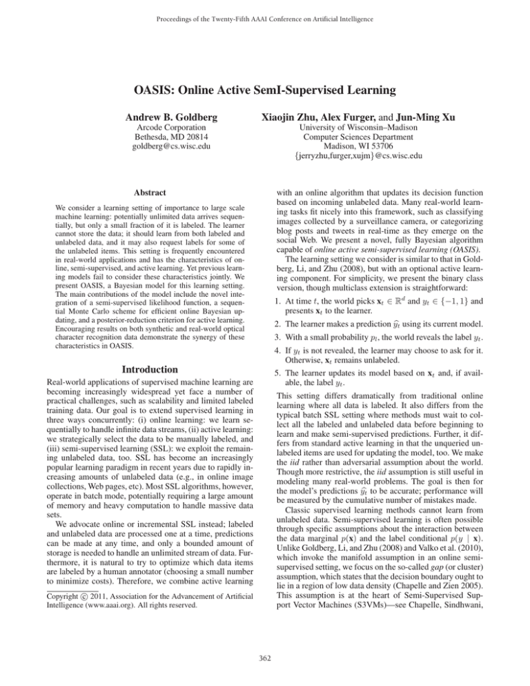
Figure 1: (a) “Null category” likelihood function to encourage low-density separation. (b) A dataset with two gaps in
unlabeled data (black dots). (c) Its bimodal posterior. S3VM
point-estimate marked by ×.
mass in the likelihood function, acting as a Bayesian analog to an SVM’s margin. Our likelihood (visualized in Figure 1(a)) is defined as follows
p(y | x, w) =
min(1 − γ, max(γα, c exp(−yc w x))) if y ∈ {−1, 1}
,
1 − [p(y = +1|x, w) + p(y = −1|x, w)] if y = ∅
where γ = 0.2, α = 0.5, c = (1 − γ)γα, c = log( γα
c ),
though other function forms leading to the same general
shape would serve our purpose, too.
This likelihood has several interesting properties, which
implement the gap assumption. It is flat beyond a margin
value (w x) of 1 or −1 to ensure that weight vectors placing data outside the margin are treated equally. Furthermore,
due to the convex curvature of the positive and negative
class likelihoods within [−1, 1], there is a concave null category probability between −1 and 1. We never receive data
from the null category; rather, unlabeled data will be considered to be in either the positive or the negative class:
p(y unlabeled | x, w) = p(y ∈ {−1, 1} | x, w) = p(y =
+1 | x, w) + p(y = −1 | x, w). Therefore, a weight vector
w that places unlabeled data x in the “null category region”
w x ∈ [−1, 1] has a lower likelihood. As a result, this likelihood favors decision boundaries that fall in a low-density
region of the input space.
To complete the model, we need to specify a prior on
the parameter w. As discussed in the experiments, we used
independent Cauchy priors on each dimension p(w) =
d
i=1 Cauchy(wi ; 0, ν) and standardized data.
With the likelihood and prior defined, we can apply Bayes
rule to derive the posterior over weight vectors (after observing past data Dt−1 ), and the predictive distribution:
t−1
i=1 p(yi | xi , w)p(w)
p(w | Dt−1 ) = t−1
(1)
i=1 p(yi | xi , w )p(w )dw
p(y | xt , w )p(w | Dt−1 )dw .(2)
p(y | xt , Dt−1 ) =
The OASIS Model
A Bayesian Model for the Gap Assumption
Recall that we observe a partially labeled sequence of feature vectors x1 , x2 , . . ., where each xt ∈ Rd . Let Dt =
{(x1 , y1 ), . . . , (xt , yt )} be all the data observed through time
t, where we use yt = 0 for unlabeled data. Our goal is to
learn a classifier to predict the class label of each incoming
unlabeled data point, and then update the classifier based on
the information we obtain (xt alone or (xt , yt )). For now,
we assume a linear classifier, but the approach can be kernelized using the randomization trick in Rahimi and Recht
(2007). Let the classifier be parametrized by weight vector
w ∈ Rd , which interacts with the data through a linear function f (x) = w x. In practice, we can handle a bias term by
adding a dummy feature to all feature vectors. Throughout,
we use the terms classifier and weight vector interchangeably. To define our Bayesian model, we begin by introducing a likelihood function that is sensitive to unlabeled data
and inspired1 by the null category noise model in Lawrence
and Jordan (2004). In addition to the positive and negative
classes, we model a third “null category” which is never
actually observed, but occupies some region of probability
1
Despite the similar appearance of the likelihood functions, the
current work is actually quite different from Lawrence and Jordan
(2004); we are concerned with the strictly online setting, and we
maintain the posterior over weight vectors through particle filtering, rather than making a Gaussian approximation which loses the
critical ability to track multiple modes in the posterior. Such posterior is typical of semi-supervised learning.
In general, it is not possible to compute this probability in
closed form. The next section describes a tractable solution.
Since we never actually predict the null category, we are ultimately interested in the following conditional probability
363
when y ∈ {−1, 1} but is unobserved:
p(y | xt , Dt−1 , y ∈ {−1, 1}) =
p(y | xt , Dt−1 )
.
p(y = −1 | xt , Dt−1 ) + p(y = 1 | xt , Dt−1 )
Input: Number of particles m, prior distribution p(w),
proposal distribution q(
w | w), threshold s0 for
active learning score function (see (6))
(1)
for t = 1, . . . do
Receive xt and possibly yt .
Active: If unlabeled, query for yt if score(xt ) < s0
To appreciate why maintaining a multimodal posterior is
desirable, consider the example data set in Figure 1(b) containing two gaps (of equal width) within the unit circle. With
a large amount of unlabeled data (black dots) and only two
labeled points (large colored symbols) in opposite wedges, a
decision boundary in either gap is feasible, and thus the posterior (Figure 1(c)) is bimodal, as indicated by the contours.
The w’s in the cone-shaped regions classify the labeled data
correctly while placing the unlabeled data outside the null
category region. Close to the origin, the w’s have magnitude too small to place all data outside the margin (since
x ≤ 1), hence the cones do not extend to the origin. The
S3VM solution corresponds to a point estimate near2 one
of the modes of the posterior. Lawrence and Jordan (2004)
will use a unimodal Gaussian approximation and miss the
posterior structure. The key to OASIS is to maintain and update an estimate of the multimodal posterior as labeled and
unlabeled data arrives.
if yt is available then update ∀i = 1 . . . m:
(i)
wi = wi p(y = yt |xt , wt−1 ).
(i)
else update wi = wi p(y ∈ {−1, 1}|xt , wt−1 ).
if effective sample size ( wi )2 / wi2 < m
2 then
Resample-Move particle filtering:
(i)
{
w }m
i=1 ← Systematic resampling
(i) m
(i)
{wt }i=1 ← Metropolis-Hastings for each w
(using proposal distribution q).
1
.
Reset particle weights wi = m
else
(i)
(i)
Keep existing particles: wt = wt−1 .
Renormalize particle weights {wi } to sum to 1.
end
end
Algorithm 1: The OASIS algorithm
Online SSL via Particle Filtering
Given the Bayesian model defined in the preceding section,
our goal is to track the posterior. In theory, this is done by
repeatedly applying Bayes rule. The integrals involved in
using the full posterior are intractable, though, so we must
resort to approximate methods. In particular, we use particle filtering with resample-move to reduce particle degeneracy (Gilks and Berzuini 2001). The complete OASIS algorithm is summarized in Algorithm 1 and explained below.
See Doucet, De Freitas, and Gordon (2001) for standard particle filtering terminology such as effective sample size and
systematic resampling.
Particle filtering is a sequential Monte Carlo technique designed for tracking and approximating distributions that are
not amenable to analytical representation (Doucet, De Freitas, and Gordon 2001). It relies on maintaining a sample of so-called particles to approximate the true distribution in question. We approximate the posterior distribution
p(w | Dt−1 ) by the empirical
mdistribution over m weighted
particles: p(w | Dt−1 ) ≈ i=1 wi δ(w − w(i) ). Each particle w(i) , i = 1 . . . m is a sample from the posterior and
has an associated importance weight wi . At time t, the
predictive distributioncan be approximated by particles as
m
(i)
P (y | xt , Dt−1 ) ≈
i=1 wi p(y | xt , w ). Recall, however, that the conditional probability
p(y | xt , Dt−1 , y ∈ {−1, 1})
m
p(y | xt , w(i) )
≈
wi
p(y = −1 | xt , w(i) ) + p(y = 1 | xt , w(i) )
i=1
For online learning, we begin by sampling m particles
from the prior and assign uniform initial weights 1/m. Then,
we repeatedly update the posterior based on the likelihood
and the previous estimate of the posterior (which now acts
as the prior). The new posterior
distribution after observing
m
xt , yt is proportional to i=1 wi p(yt | xt , w(i) )δ(w − w(i) ).
We represent the new posterior by reweighting the particles.
From the above equation, we see that the new weight for w(i)
is obtained as the current weight multiplied by the likelihood
p(yt | xt , w(i) ). If yt is unlabeled, the weight is multiplied
by p(yt ∈ {−1, 1} | xt , w(i) ) = 1 − p(yt = ∅ | xt , w(i) ).
So far we have a basic method for incrementally updating an approximate posterior after observing new data.
Classic particle methods, such as sampling importance resampling (SIR) (Doucet and Johansen 2009), use the particle weights for resampling (with replacement). While theoretically justified, repeating this process many times is
known to cause particle degeneracy—the number of distinct
particles is non-increasing, so eventually few will remain.
To minimize particle degeneracy, we apply the resamplemove algorithm (Gilks and Berzuini 2001), which provides
a principled way to “jitter” particles and introduce diversity into the pool. Following a resampling step, particles are
potentially relocated by applying one step of MetropolisHastings (Metropolis et al. 1953; Hastings 1970). Using a
symmetric proposal distribution q(
w | w) allows us to compute the acceptance probability for each move using only the
(4)
is used to make predictions for incoming data.
2
(m)
Sample initial particles w0 . . . w0 ∼ p(w).
1
, i = 1, . . . , m.
Assign initial particle weights wi = m
(3)
They do not overlap because their loss functions differ.
364
unnormalized posterior f (w | Dt ):
(i)
f (
w | Dt ) (i)
,
α(
w , w(i) ) = min 1,
f (w(i) | Dt )
points are ignored (no SSL). Adapting the theory to account
for the semi-supervised updates between active queries remains an open issue for future work.
(5)
Empirical Evaluation
(i)
is a proposed move, and f (w | Dt ) =
where w
t
p(w) k=1 p(yk | xk , w), where yk is understood to be
{−1, 1} for unlabeled data.
We conducted a series of experiments on OASIS. We carefully tease apart OASIS’s different elements and show
that active online querying leads to better performance
than random online labeling, in the context of online
semi-supervised learning. Furthermore, the use of semisupervised learning in the online setting (even without active querying) often outperforms the identical learner that
ignores unlabeled data, as well as a state-of-the-art online
supervised learner.
For all experiments, to avoid difficult parameter tuning
under online semi-supervised conditions, we use the same
prior and proposal distributions with a fixed set of hyperparameters. Following Gelman et al. (2008), we standardize the data so each feature has mean 0 and standard deviation 0.5, and place independent Cauchy(0, 2.5) priors
on each dimension. For the proposal distribution, we use a
more peaked version of this distribution: Cauchy(0, 0.025).
All experiments use m = 1000 particles with buffer size
τ = 100.
The experiments consider five algorithms:
1. [OASIS]: Algorithm 1
2. [OSIS]: Online and semi-supervised; no active learning,
but otherwise the same as OASIS.
3. [OS]: Online and supervised; no active learning or SSL.
4. [AROW (C = 1)]: State-of-the-art supervised “Adaptive
Regularization of Weight Vectors” online learner (Crammer, Kulesza, and Dredze 2009), run using code provided
by the original authors with a default regularization parameter C = 1. This is a passive-aggressive, confidenceweighted classifier that maintains a diagonal-covariance
Gaussian distribution over weight vectors.
5. [AROW (C ∗ )]: We also report results for AROW using
the per-trial clairvoyant C in terms of total number of mistakes (“test-set tuned”) to approximate supervised learning’s mistake lower bound.
We use the following experimental procedure to compare
active and passive algorithms, with and without the help of
unlabeled data. Each experiment is based on 20 random trials of randomized sequences of T points. Each trial begins
with l = 2 labeled examples (one per class, in random order), as we assume this is practical. While OASIS is the only
algorithm under consideration that can actively query labels,
we take care to ensure that each algorithm receives exactly
the same total number of labels. Let a be the number of active queries OASIS makes on a given trial, determined by
the active querying threshold s0 and the data set. For each
trial, we do the following: (i) Run OASIS with l = 2 initial
labels and record a (number of queries); (ii) Run each other
algorithm with l = 2 + a labeled examples (first two, plus a
randomly selected others). Note the same exact sequence of
{xt } vectors is used across the same trial for different algorithms. In this way, all algorithms always see the same data
Constant Time and Space Complexity Per Iteration
Computing (5) in the “move” step requires access to the entire history of data Dt , which is infeasible for learning on
an unlimited stream of data. Thus, we propose using an approximate Metropolis-Hastings step in which the acceptance
probability is computed using only a fixed-length buffer of
size τ . That is, we replace f (w | Dt ) with f (w | Dt , τ ) =
t
p(w) k=t−τ +1 p(yk | xk , w). While this approximation is
different from the true posterior, it has constant time and
space complexity and will be shown to be effective in practice. In addition, though not explored in the current work, using a τ -buffer can allow the method to handle concept drift
by only relying on the most recent sample of data.
Even with a τ -buffer, computing the Metropolis-Hastings
acceptance probability for each particle can be computationally intensive. Therefore, we only perform resample-move
when
so-called Effective Sample Size—estimated by
the ( wi )2 / wi2 —drops below m/2, as is customary in the
literature (Doucet and Johansen 2009; Ridgeway and Madigan 2003). Otherwise, the algorithm proceeds to the next
time step with the same particles reweighted.
Incorporating Active Learning
It is quite natural to incorporate online active learning into
the algorithm described thus far. The posterior can be viewed
as a soft version space, and like many active learning algorithms, we select queries that will maximally pare down the
version space. In our case, we query items that will lead to
downweighting and effectively killing off many particles.
To determine whether to query the label of an incoming unlabeled item x, we compute its disagreement
score (Nowak 2009) using the current particles:
m
(i) (6)
wi argmax p(y | x, w ) .
score(x) = y∈{−1,1}
i=1
This score is close to zero if roughly half of the particles predict positive and half negative. Querying the label of such
an item is beneficial, as roughly half of the particles (whose
predictions disagree with the oracle label) will get downweighted.
While many schemes are possible to balance the trade-off
between the cost of acquiring a label and the benefit of refining the model, we use a simple thresholding approach in
the current work. Actively querying points that minimize the
score criterion in (6) is theoretically justified in a pool-based
active learning setting (Nowak 2009). The same theory can
also be applied to the online active setting to justify a constant threshold. However, that analysis assumes unqueried
365
dicedcube2, ¡=0.1
slicedcube2, ¡=0.1
0.4
0.4
0.3
0.3
0.2
0.2
0.1
0.1
0
0
0.1
0.1
0.2
0.2
0.3
0.3
0.4
0.4
0.6
world optical character recognition (OCR) tasks through
their use of active sampling and online updates based on
unlabeled data. We used the MNIST dataset3 and two UCI
datasets, letter and pendigits.
On all three data sets, Figure 4 shows a clear ordering of performance: active SSL is better than passive SSL
is better than passive supervised learning. We can measure statistically significant performance differences by applying two-sample t-tests to the total numbers of mistakes
made by pairs of algorithms across the 20 trials.4 On letter, OASIS significantly outperforms all the supervised algorithms (p < 0.05), and makes fewer mistakes than the
passive semi-supervised OSIS. OSIS fails to achieve statistical significance at the 0.05 level over the supervised baselines, suggesting that for this task, OASIS’s active learning
(rather than the use of unlabeled data) gives it the advantage.
On pendigits and MNIST, though, both OASIS and OSIS
make significantly fewer mistakes overall than each of the
three supervised learners. Furthermore, on MNIST, OASIS
significantly beats OSIS, demonstrating that actively queried
labels can be more useful than randomly sampled labels in
the context of online semi-supervised learning.
0.4
0.2
0
0.2
0.4
0.6
(a) sliced-cube-2 data
0.6
0.4
0.2
0
0.2
0.4
0.6
(b) diced-cube-2 data
Figure 2: Sliced-cube and diced-cube synthetic data sets.
and the same total number of labels; the algorithms differ in
exactly which labels and how they deal with unlabeled data.
All experiments were implemented in MATLAB and ran
quickly on a modern processor. The average per-iteration run
times for each method (over 20 trials and all data sets) were:
OS 2.3ms, OSIS 3.8ms, OASIS 4.0ms, AROW C = 1 and
C ∗ 0.1ms. Note the OS, OSIS, and OASIS code was not
optimized for speed.
Synthetic Data
We begin by considering two families of synthetic data sets:
• sliced-cube-d: Uniformly distributed unit cube in
[−0.5, 0.5]d , with an -width slab removed from the first
dimension to create two hyper-rectangles with a gap
around the true decision boundary x1 = 0 (Figure 2(a)).
• diced-cube-d: Same as sliced-cube-d (with true decision
boundary x1 = 0), except -width slabs are removed from
all dimensions to create 2d hypercubes separated by potentially misleading low-density gaps (Figure 2(b)).
For both data sets, = (T /10)−1/d , such that the gaps
should be large enough (relative to the average spacing between points) to be detectable after T /10 points (Singh,
Nowak, and Zhu 2008).
Figure 3 plots the 20-trial average cumulative number of
mistakes made by each algorithm when predicting the label
of each incoming data point (regardless of whether the label
ends up being revealed naturally or actively queried). The
captions indicate the mean and standard deviation of a, the
number of additional labels used in learning (via active selection for OASIS and random selection for the baselines).
We observe that OASIS very quickly learns the true decision
boundary and stops making mistakes across both data sets
for all dimensionalities considered (d ∈ {2, 4, 8, 16, 32},
though only d = 2 and d = 32 are shown here). As expected, active querying allows OASIS to resolve ambiguities
between the multiple gaps in the diced-cube-d data, though
learning the decision boundary in this more confusing case
takes longer on average. Comparing OSIS to OS and both
versions of AROW, we see that SSL provides a large advantage, even when the few labeled data points are randomly
selected. This example provides a proof of concept for the
particle filtering approach to tracking the posterior, both in
cases where the data distribution satisfies the gap assumption and when it contains misleading gaps.
Conclusions and Future Work
We have presented a Bayesian learning model, OASIS,
which combines online learning, semi-supervised learning,
and active learning. OASIS exploits unlabeled data through
the low-density gap assumption and is able to avoid the
non-convex optimization typically associated with similar
SSL algorithms by maintaining an approximation of the
posterior over weight vectors via particle filtering. Outside of some special-purpose classifiers for computer vision
tracking applications (Grabner, Leistner, and Bischof 2008;
Tang et al. 2007), few authors have examined the task of online semi-supervised learning. The OASIS model presented
here also integrates active learning and shows significant improvements over passive supervised baselines on both synthetic and real-world data.
Our experiments focused on relatively low dimensional
data sets. It is well-known that particle filtering and sequential Monte Carlo techniques can be less efficient in high dimensions. One way to adapt OASIS to better handle much
higher dimensional data sets, including those resulting from
random-feature-based kernelization, is to improve the proposal distribution in the MCMC step of resample-move. The
current approach uses a symmetric random walk proposal
distribution q, which limits the ability of particles to jump
between modes in the posterior. It is possible that we can
achieve better mixing by adapting the proposal distribution
based on the previous set of particles.
Future work will also examine alternative active learning
strategies, especially ones that strictly limit the total number
3
For the MNIST data, we reduced the dimensionality down
to 10 via “online PCA.” To roughly simulate the online setting,
principal components were found based on x1 , . . . , x1000 , and
x1001 , . . . , x10000 were simply projected into the resulting space.
4
The specific labeled examples differ between OASIS and the
passive algorithms, so the samples are not paired.
Real-World Data
We next demonstrate that OASIS and its passive counterpart
OSIS significantly outperform supervised baselines on real-
366
0
50
0
0
200
400
600
800
0
200
100
0
0
1000
t
200
400
600
800
100
0
50
0
0
1000
200
400
600
800
300
AROW (C=1)
*
AROW (C )
OS
OSIS
OASIS (s =0.01)
0
200
100
0
0
1000
200
400
t
t
(a) sliced-cube-2
a = 0.25(0.44)
400
AROW (C=1)
*
AROW (C )
OS
OSIS
OASIS (s =0.01)
20trial mean
cumulative #mistakes
100
300
150
AROW (C=1)
*
AROW (C )
OS
OSIS
OASIS (s =0.01)
20trial mean
cumulative #mistakes
400
AROW (C=1)
*
AROW (C )
OS
OSIS
OASIS (s =0.01)
20trial mean
cumulative #mistakes
20trial mean
cumulative #mistakes
150
(b) sliced-cube-32
a = 4.6(0.75))
600
800
1000
t
(c) diced-cube-2
a = 0.4(0.50))
(d) diced-cube-32
a = 4.85(0.75))
Figure 3: Sliced-cube-d and diced-cube-d synthetic data results for T = 1000, l = 2, s0 = 0.01.
100
80
120
AROW (C=1)
*
AROW (C )
OS
OSIS
OASIS (s =0.01)
0
60
40
20
500
1000
1500
t
(a) letter A vs B (d = 16)
T = 1555, l = 2, a = 5.10(1.92)
100
80
300
AROW (C=1)
*
AROW (C )
OS
OSIS
OASIS (s =0.01)
20trial mean
cumulative #mistakes
120
20trial mean
cumulative #mistakes
20trial mean
cumulative #mistakes
140
0
60
40
20
500
1000
t
1500
2000
(b) pendigits 0 vs 1 (d = 16)
T = 2286, l = 2, a = 2.60(1.14)
250
200
AROW (C=1)
*
AROW (C )
OS
OSIS
OASIS (s =0.10)
0
150
100
50
2000
4000
6000
8000 10000
t
(c) MNIST 0 vs 1 (d = 10)
T = 10000, l = 2, a = 10.30(5.01)
Figure 4: Results on real-world OCR data. Note: s0 = 0.01 for letter and pendigits; s0 = 0.1 for MNIST.
of active queries or consider costs associated with certain
labels. The current fixed threshold strategy may not be suitable under all real-world constraints. While we could simply
impose a hard limit on the number of queries, more sophisticated approaches may be possible that delicately balance the
trade-off between asking for another label versus receiving
another unlabeled data point. In both cases, we learn something, but it may be advantageous to delay querying until
a more valuable point comes along. Many adaptive thresholding and selection criteria are possible for online active
learning (see Beygelzimer, Dasgupta, and Langford (2009)
and the references therein), and careful modification to account for the role and impact of unlabeled data could lead to
improved learning rates.
Furao, S.; Sakurai, K.; Kamiya, Y.; and Hasegawa, O. 2007. An online semi-supervised active learning algorithm with self-organizing
incremental neural network. In IJCNN.
Gelman, A.; Jakulin, A.; Pittau, M. G.; and Su, Y.-S. 2008. A
weakly informative default prior distribution for logistic and other
regression models. Annals of Applied Statistics 2(4):1360–1383.
Gilks, W. R., and Berzuini, C. 2001. Following a moving target—
Monte Carlo inference for dynamic Bayesian models. Journal Of
The Royal Statistical Society Series B 63(1):127–146.
Goldberg, A. B.; Li, M.; and Zhu, X. 2008. Online manifold regularization: A new learning setting and empirical study. In ECML
PKDD.
Grabner, H.; Leistner, C.; and Bischof, H. 2008. Semi-supervised
on-line boosting for robust tracking. In ECCV.
Hastings, W. 1970. Monte Carlo sampling methods using Markov
chains and their applications. Biometrika 57:97–109.
Lawrence, N. D., and Jordan, M. I. 2004. Semi-supervised learning
via Gaussian processes. In NIPS 17.
Metropolis, N.; Rosenbluth, A. W.; Rosenbluth, M. N.; Teller,
A. H.; and Teller, E. 1953. Equation of state calculations by fast
computing machines. Journal of Chemical Physics 21:1087–1092.
Nowak, R. 2009. Noisy generalized binary search. In NIPS 22.
Rahimi, A., and Recht, B. 2007. Random features for large-scale
kernel machines. In NIPS 20.
Ridgeway, G., and Madigan, D. 2003. A sequential Monte Carlo
method for Bayesian analysis of massive datasets. Journal of Data
Mining and Knowledge Discovery 7(3):301–319.
Singh, A.; Nowak, R.; and Zhu, X. 2008. Unlabeled data: Now it
helps, now it doesn’t. In NIPS 21.
Tang, F.; Brennan, S.; Zhao, Q.; and Tao, H. 2007. Co-tracking
using semi-supervised support vector machines. In ICCV.
Valko, M.; Kveton, B.; Huang, L.; and Ting, D. 2010. Online
semi-supervised learning on quantized graphs. In UAI.
Acknowledgments This work is supported in part by NSF
IIS-0916038, AFOSR FA9550-09-1-0313, and NSF IIS0953219. We also thank Rob Nowak for helpful discussions.
References
Beygelzimer, A.; Dasgupta, S.; and Langford, J. 2009. Importance
weighted active learning. In ICML.
Chapelle, O., and Zien, A. 2005. Semi-supervised classification by
low density separation. In AISTAT 2005.
Chapelle, O.; Sindhwani, V.; and Keerthi, S. S. 2008. Optimization
techniques for semi-supervised support vector machines. JMLR
9(Feb):203–233.
Crammer, K.; Kulesza, A.; and Dredze, M. 2009. Adaptive regularization of weight vectors. In NIPS 22.
Doucet, A., and Johansen, A. M. 2009. A tutorial on particle filtering and smoothing: Fifteen years later. In Crisan, D., and Rozovsky, B., eds., Handbook of Nonlinear Filtering. Oxford University Press.
Doucet, A.; De Freitas, N.; and Gordon, N., eds. 2001. Sequential
Monte Carlo methods in practice.
367