Proceedings of the Twenty-Fifth AAAI Conference on Artificial Intelligence
Controlling Selection Bias in Causal Inference
Elias Bareinboim and Judea Pearl
Cognitive Systems Laboratory
Department of Computer Science
University of California, Los Angeles
Los Angeles, CA. 90095
{eb,judea} at cs.ucla.edu
Abstract
Selection bias, caused by preferential exclusion of units
(or samples) from the data, is a major obstacle to valid
causal inferences, for it cannot be removed or even detected by randomized experiments. This paper highlights several graphical and algebraic methods capable of mitigating and sometimes eliminating this bias.
These nonparametric methods generalize and improve
previously reported results, and identify the type of
knowledge that need to be available for reasoning in the
presence of selection bias.
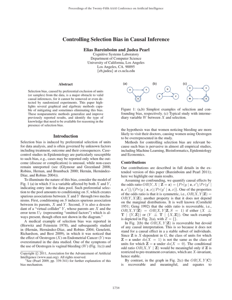
Figure 1: (a,b) Simplest examples of selection and confounding bias, respectively. (c) Typical study with intermediary variable W between X and selection.
the hypothesis was that women noticing bleeding are more
likely to visit their doctors, causing women using Oestrogen
to be overrepresented in the study.
Methods for controlling selection bias are relevant because such bias is pervasive in almost all empirical studies,
including Machine Learning, Bioinformatics, Epidemiology
and Economics.
Introduction
Selection bias is induced by preferential selection of units
for data analysis, and is often governed by unknown factors
including treatment, outcome and their consequences. Casecontrol studies in Epidemiology are particularly susceptible
to such bias, e.g., cases may be reported only when the outcome (disease or complication) is unusual, while non-cases
remain unreported (see (Glymour and Greenland 2008;
Robins, Hernan, and Brumback 2000; Hernán, HernándezDı́az, and Robins 2004)).
To illuminate the nature of this bias, consider the model of
Fig. 1 (a) in which S is a variable affected by both X and Y ,
indicating entry into the data pool. Such preferential selection to the pool amounts to conditioning on S, which creates
spurious associations between X and Y through two mechanisms. First, conditioning on S induces spurious association
between its parents, X and Y . Second, S is also a descendant of a “virtual collider” Y , whose parents are X and the
error term UY (representing “omitted factors”) which is always present, though often not shown in the diagram.1
A medical example of selection bias was reported in
(Horwitz and Feinstein 1978), and subsequently studied
in (Hernán, Hernández-Dı́az, and Robins 2004; Geneletti,
Richardson, and Best 2009), in which it was noticed that
the effect of Oestrogen (X) on Endometrial Cancer (Y ) was
overestimated in the data studied. One of the symptoms of
the use of Oestrogen is vaginal bleeding (W ) (Fig. 1(c)) and
Contributions
Our contributions are described in full details in the extended version of this paper (Bareinboim and Pearl 2011);
here we highlight our main results.
Assuming no confounding, we quantify
causal effects by
the odds
ratio
OR(Y,
X
|
Z
=
z)
=
P
r(y
| z, x )/P r(y |
z, x ) / P r(y | z, x)/P r(y | z, x) . One of the properties
of the odds ratio is that it is symmetric, i.e., OR(X, Y |Z) =
OR(Y, X|Z); another property is that it does not depend
on the marginal distributions. It is well known (Cornfield
1951; Geng 1992) that the odds ratio is recoverable, i.e.,
OR(X, Y |Z) = OR(X, Y |Z, S = 1) if either (X ⊥⊥
T | {Y, Z}) or (Y ⊥⊥ T | {X, Z}). One such example
is depicted in Fig. 2(a), with Z = {}.
In Fig. 2(b) the OR(X, Y |Z) is recoverable but devoid
of any causal interpretation. This is so because it does not
stand for a causal effect in a a stable subset of individuals.
Since Z is X-dependent in G, the class of units for which
Z = z under do(X = 1) is not the same as the class of
units for which Z = z under do(X = 0). The conditional
odd ratio OR(X, Y | Z) would be meaningful only if Z is
restricted to pre-treatment covariates, which are X-invariant,
hence stable.
By contrast, in the graph in Fig. 2(c) the OR(X, Y |C)
is recoverable and meaningful, and equates to
c 2011, Association for the Advancement of Artificial
Copyright Intelligence (www.aaai.org). All rights reserved.
1
See (Pearl 2009, pp. 339-341) for further explanation of this
bias mechanism.
1754
(iii) the dimensionality of Z matches the dimensionality of
{X, Y }; (iv) the marginal distribution of Z is known.
This result is surprising for two reasons: first, we generally do not expect selection bias to be removable; second,
bias removal in the presence of confounding is generally expected to be a more challenging task. We finally show how
this result is applicable to scenarios where other structural
assumptions hold, for instance, when an instrument is not
available but a certain back-door admissible set can be identified (Bareinboim and Pearl 2011, Corol. 3–5).
Figure 2: (a) Chain graph representing case-control study
where the OR(X, Y ) is recoverable. (b) Scenario where the
OR(X, Y | Z) is recoverable but meaningless. (c) Example
where the c-specific OR is recoverable and meaningful.
Conclusion
We showed that qualitative knowledge of the selection
mechanism together with graphical and algebraic methods
can eliminate selection bias in many realistic problems. In
particular, the paper provides a simple graphical condition,
together with an algorithm to decide, given a DAG with measured and unmeasured variables, whether and how a given
c-specific odds ratio can be recovered from selection-biased
data. We further showed by algebraic methods that selection
bias can be removed in the presence of confounding with the
help of instrumental variables under certain mild conditions.
OR(X, Y |C, W, S = 1). The following theorem provides a general graphical condition under which the
population odds ratio (OR) or a covariate-specific causal
odds ratio can be recovered from selection-biased data:
Theorem 1 (Bareinboim and Pearl 2011, Thm. 2) Let
graph G contain the arrow X → Y and a selection node
S. A necessary and sufficient condition for G to permit the
G-recoverability of OR(Y, X | C) for some set C of pretreatment covariates is that every ancestor Ai of S that is
also a descendant of X have a separating set Ti that either
d-separates Ai from X given Y , or d-separates Ai from Y
given X. (We define S to be among its ancestors).
Moreover, if the condition above holds, then OR(Y, X |
C) is G-recoverable if C d-separates Y (given X) from all
pre-treatment variables that are invoked in at least one Ti ,
and it equals OR(Y, X | C, T, S = 1), where T = i Ti .
For instance, the problem studied in (Geneletti, Richardson, and Best 2009) (Fig. 1(c)) is trivially solved by the Theorem 1, yielding OR(X, Y ) = OR(X, Y | W, S = 1).
Having characterized recoverability of the odds ratio, we
studied universal curves that show the behavior of OR as the
distribution P (y | x) changes, and how other measures of
association such as risk ratio (RR) and risk difference (RD)
are related to OR. We further showed that if one is interested
in recovering RR and RD under selection bias, knowledge of
the marginal distribution P (X) is sufficient for recovery.
The results stated so far focus on point identifiability for
the quantity of interest, but there are abundant scenarios
where causal effects are non-identifiable and selecion bias
can simultaneously be present, further increasing the bias.
One of the methods used to cope with non-identifiability
is to bound the causal effecs through instrumental variables
(Pearl 2009, Ch. 8), but since the bounding analysis assumes
no selection bias, the question arises whether tighter bounds
can be derived in the presence of selection bias.
We show that selection bias can be removed entirely
through the use of IVs, therefore, the bounds on the causal
effect will be narrower than those obtained under the
selection-free assumption as follows:
Theorem 2 (Bareinboim and Pearl 2011, Corol. 3) The
bounds for the causal effect of X on Y can be recovered
from selection bias whenever the following conditions hold:
(i) the S node is affected by the set Z only through {X, Y };
(ii) the set Z is d-connected to {X, Y } (and combinations);
Acknowledgment
This paper benefited from discussions with Onyebuchi Arah
and Sander Greenland. This research was supported in parts
by NIH #1R01 LM009961-01, NSF #IIS-0914211 and #IIS1018922, and ONR #N000-14-09-1-0665 and #N00014-101-0933.
References
Bareinboim, E., and Pearl, J.
2011.
Controlling selection bias in causal inference.
Technical Report R381, <http://ftp.cs.ucla.edu/pub/stat ser/r381.pdf>, Department of
Computer Science, University of California, Los Angeles.
Cornfield, J. 1951. A method of estimating comparative rates from
clinical data; applications to cancer of the lung, breast, and cervix.
Journal of the National Cancer Institute 11:1269–1275.
Geneletti, S.; Richardson, S.; and Best, N. 2009. Adjusting for
selection bias in retrospective, case-control studies. Biostatistics
10(1).
Geng, Z. 1992. Collapsibility of relative risk in contingency tables with a response variable. Journal Royal Statistical Society
54(2):585–593.
Glymour, M., and Greenland, S. 2008. Causal diagrams. In Rothman, K.; Greenland, S.; and Lash, T., eds., Modern Epidemiology.
Philadelphia, PA: Lippincott Williams & Wilkins, 3rd edition. 183–
209.
Hernán, M.; Hernández-Dı́az, S.; and Robins, J. 2004. A structural
approach to selection bias. Epidemiology 15(5):615–625.
Horwitz, R., and Feinstein, A. 1978. Alternative analytic methods
for case-control studies of estrogens and endometrial cancer. New
England Journal of Medicine 299:368–387.
Pearl, J. 2009. Causality: Models, Reasoning, and Inference. New
York: Cambridge University Press, 2nd edition.
Robins, J. M.; Hernan, M.; and Brumback, B. 2000. Marginal
structural models and causal inference in epidemiology. Epidemiology 11(5):550–560.
1755