Proceedings of the Twenty-Sixth AAAI Conference on Artificial Intelligence
Bayesian Unification of Sound Source Localization
and Separation with Permutation Resolution
Takuma Otsuka† , Katsuhiko Ishiguro‡ , Hiroshi Sawada‡ , and Hiroshi G. Okuno†
†Graduate School of Informatics, Kyoto University, Kyoto, 606-8501, Japan.
{ohtsuka, okuno}@kuis.kyoto-u.ac.jp
‡NTT Communication Science Laboratories, NTT Corporation, Kyoto, 619-0237, Japan.
{ishiguro.katsuhiko, sawada.hiroshi}@lab.ntt.co.jp
Abstract
Sound source localization and separation with permutation resolution are essential for achieving a computational auditory scene analysis system that can extract
useful information from a mixture of various sounds.
Because existing methods cope separately with these
problems despite their mutual dependence, the overall
result with these approaches can be degraded by any
failure in one of these components. This paper presents
a unified Bayesian framework to solve these problems
simultaneously where localization and separation are
regarded as a clustering problem. Experimental results
confirm that our method outperforms state-of-the-art
methods in terms of the separation quality with various
setups including practical reverberant environments.
1
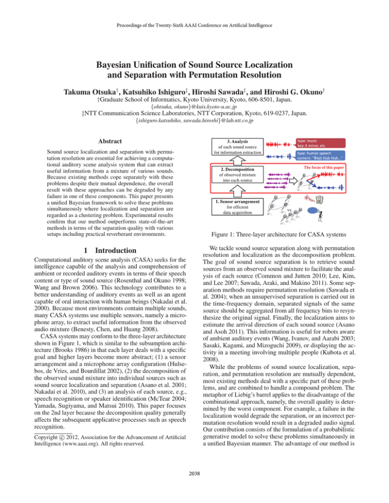
Figure 1: Three-layer architecture for CASA systems
We tackle sound source separation along with permutation
resolution and localization as the decomposition problem.
The goal of sound source separation is to retrieve sound
sources from an observed sound mixture to facilitate the analysis of each source (Common and Jutten 2010; Lee, Kim,
and Lee 2007; Sawada, Araki, and Makino 2011). Some separation methods require permutation resolution (Sawada et
al. 2004); when an unsupervised separation is carried out in
the time-frequency domain, separated signals of the same
source should be aggregated from all frequency bins to resynthesize the original signal. Finally, the localization aims to
estimate the arrival direction of each sound source (Asano
and Asoh 2011). This information is useful for robots aware
of ambient auditory events (Wang, Ivanov, and Aarabi 2003;
Sasaki, Kagami, and Mizoguchi 2009), or displaying the activity in a meeting involving multiple people (Kubota et al.
2008).
While the problems of sound source localization, separation, and permutation resolution are mutually dependent,
most existing methods deal with a specific part of these problems, and are combined to handle a compound problem. The
metaphor of Liebig’s barrel applies to the disadvantage of the
combinational approach, namely, the overall quality is determined by the worst component. For example, a failure in the
localization would degrade the separation, or an incorrect permutation resolution would result in a degraded audio signal.
Our contribution consists of the formulation of a probabilistic
generative model to solve these problems simultaneously in
a unified Bayesian manner. The advantage of our method is
Introduction
Computational auditory scene analysis (CASA) seeks for the
intelligence capable of the analysis and comprehension of
ambient or recorded auditory events in terms of their speech
content or type of sound source (Rosenthal and Okuno 1998;
Wang and Brown 2006). This technology contributes to a
better understanding of auditory events as well as an agent
capable of oral interaction with human beings (Nakadai et al.
2000). Because most environments contain multiple sounds,
many CASA systems use multiple sensors, namely a microphone array, to extract useful information from the observed
audio mixture (Benesty, Chen, and Huang 2008).
CASA systems may conform to the three-layer architecture
shown in Figure 1, which is similar to the subsumption architecture (Brooks 1986) in that each layer deals with a specific
goal and higher layers become more abstract; (1) a sensor
arrangement and a microphone array configuration (Hulsebos, de Vries, and Bourdillat 2002), (2) the decomposition of
the observed sound mixture into individual sources such as
sound source localization and separation (Asano et al. 2001;
Nakadai et al. 2010), and (3) an analysis of each source, e.g.,
speech recognition or speaker identification (McTear 2004;
Yamada, Sugiyama, and Matsui 2010). This paper focuses
on the 2nd layer because the decomposition quality generally
affects the subsequent applicative processes such as speech
recognition.
c 2012, Association for the Advancement of Artificial
Copyright Intelligence (www.aaai.org). All rights reserved.
2038
in that it both solves the multiple problems and improves the
separation quality by incorporating a localization estimate.
2
Problem statement and issues
This section presents the problem dealt with in this paper,
three issues, and the need for a unified framework. The decomposition
problem is summarized as follows:
Input: Multichannel audio signal,
Outputs: The direction of arrival and separated signal
of each sound source,
Assumptions: The microphone array configuration is
known as steering vectors, the number of sources is
given, and the sound source directions do not change
over time.
A steering vector conveys the time difference of sound arrivals at each sensor given a certain direction of the sound
source and a frequency bin. Our implementation uses steering
vectors measured in an anechoic chamber. Thus, our method
works independently of the environment. The number of
sources is important especially in reverberant environments
where automatic estimation is still a challenge. Some alleviation of these assumptions is discussed in Section 5.
The issues are threefold; (1) permutation resolution with
frequency domain processing, (2) underdetermined conditions where the number of sources exceeds the number of
sensors, and (3) distinguishable sound source selection.
Three issues First, most environments contain reverberation modeled as a convolutive mixture (Pedersen et al. 2007).
Microphone array processing in the frequency domain copes
with this situation. Although this strategy can handle the reverberation by converting the convolution into element-wise
multiplications through a Fourier transform, the permutation
problem (Sawada et al. 2004) is induced.
The permutation problem occurs when the separation is
carried out independently of each frequency bin in an unsupervised manner, for example using independent component
analysis (ICA) (Common and Jutten 2010). When we aggregate the spectrogram of a certain source, we must identify
signals of the same sound source from all frequency bins.
Independent vector analysis (IVA) (Lee, Kim, and Lee 2007;
Ono 2011) avoids the permutation problem by maximizing
the independence of constituent sound sources across all
frequency bins at the same time.
Second, some linear mixture models including ICA and
IVA assume that the number of sources N does not exceed
the number of microphones M . In practice, however, N is not
always guaranteed to be capped at M . The case where N >
M is called an underdetermined condition. While Sawada
et al. (2011) cope with the underdetermined condition by
the frequency-wise clustering of sound sources, their method
requires permutation resolution after the clustering. This twostep strategy may degrade the overall separation quality.
The third issue is typically related to linear mixture models
such as IVA (Lee, Kim, and Lee 2007; Ono 2011). In many
cases, we have to select N distinct sound sources from among
the M separated signals because in practice we often set
M > N to avoid underdetermined conditions. A failure in
this selection step would degrade the separation itself as well
as any subsequent analysis such as speech recognition.
The IVA algorithm simply decomposes an observed mixture consisting of M channels into M independent signals.
In many cases, IVA is applied where M > N . Thus, we
have to reduce the dimensionality M to N by employing, for
example, principal component analysis as a preprocessing.
Towards a unified framework As explained in Section 1,
the relationship between sound source localization, separation, and the permutation resolution obeys the Liebig’s Law.
For example, (Nakadai et al. 2010) achieves both localization and separation by solving each problem in order; after
localizing each sound, each sound source is extracted by
emphasizing signals coming from the estimated directions.
This method is advantageous in that the separation avoids the
permutation resolution because each source can be specified
by its direction. Here, incorrect localization would result in
degraded separation quality. The localization with IVA is
another example: The correlation of the separated signals and
steering vectors is investigated for the localization. Here, the
localization process is sensitive to the preceding separation.
Two major solutions have been proposed for the permutation problem (Sawada et al. 2004). One involves synchronizing the change in the power envelope of a source over
frequency bins. The other involves combining the separated
signals estimated to come from the same direction. Both
methods can degrade the outcome due to permutation errors
by incorrect frequency-wise separation or localization.
Our method unifies all the problems into a Bayesian framework. The separation and localization problem is formulated
as a clustering problem in the time-frequency domain. Permutation resolution employs both the above ideas: 1) We
introduce a sound dominance proportion for each time frame
to encourage each sound source to synchronously increase
its power over frequency bins. 2) The direction is used to
identify the separated signals at each frequency bin.
3
Method
Figure 2 outlines our method. First, the mixed signal to be
observed is generated by adding sound sources as shown on
the left in Fig. 2. A real-valued waveform in the time domain is converted into complex values in the time-frequency
domain by a short-time Fourier transform (STFT). Then, a
time-frequency mask (TF mask) is estimated for each source
to retrieve it from the mixture.
Figure 2 shows power spectrograms on a linear scale to
emphasize that the power is sparsely distributed in the timefrequency domain, that is, the power is nearly zero at most
time-frequency points. Therefore, we can assume that only
one sound source is dominant at each time-frequency point
and that we are able to extract sound sources with TF masks.
The estimation of the TF masks is formulated as a clustering problem on the observed multi-channel signal in the
time-frequency domain. Each time-frequency point stems
from a certain source referred to as a class in the clustering
context. Our method estimates the posterior probability to
which class each time-frequency point belongs. Furthermore,
2039
Figure 2: Illustration of mixture process and separation method based on time-frequency masking
where ·H means a Hermitian transpose.
As shown in Figure 3, the covariance matrix of each source
has an eigenvector with a salient eigenvalue. This vector corresponds to the steering vector associated with the direction
in which the source is located. That is, the clustering of each
sample corresponds to the separation of sound sources, and
the investigation of the eigenvectors of the clustered covariances means the localization of sources.
The covariance is factorized into a power term and a steering matrix. While the power of the signal |stf k |2 is timevarying in Eq. (1), the steering term qf d qH
f d is fixed over
time since we assume steady sources. Because we can assume st,f,k and qf d are independent, we introduce an inverse power λtf k ≈ |stf k |−2 and an inverse steering matrix
−1
Hf d ≈ (qf d qH
, where IM is the M ×M identity
f d +IM )
matrix. The likelihood
distribution
is
Y
p(x̃|z̃, w̃, λ̃, H̃) =
NC (xt f |0, (λtf k Hf d )−1 )ztf k wkd ,
our method handles more classes than the actual number of
sound sources for the clustering to make our algorithm independent of the number of actual sound sources. We set
parameters s.t. redundant classes shrink during the clustering
and we obtain stable results regardless of the source number.
Our method resembles (Mandel, Ellis, and Jebara 2007)
in that time-frequency points are clustered into each source
to generate TF masks. While Mandel et al. use only the
phase of complex values and 2 microphones, our method
uses the complex values themselves and allows 2 or more
microphones that produce better results.
Sections 3.1–3.3 explain the generative process and Section 3.4 presents the inference procedures. Table 1 shows the
notations we use. A set of variables is denoted with a tilde
without subscripts, e.g., x̃ = {xtf |1 ≤ t ≤ T, 1 ≤ f ≤ F }.
Table 1: Notations
tf kd
Symbol
t
f
k
d
M
N
xtf
ztf
πt
wk
ϕ
λtf k
Hf d
3.1
Meaning
Time frame ranging from 1 to T
Frequency bin from 1 to F
Class index from 1 to K
Direction index from 1 to D
Number of microphones
Number of sound sources
Observed M -dimensional complex column vector
Class indicator at t and f
Class proportion at time t
Direction indicator for class k
Direction proportion for all classes
Inverse power of class k at t and f
Inverse covariance of direction d at frequency f
(2)
|Λ|
(2π)M
exp −xH Λx is the probwhere NC (x|µ, Λ−1 ) =
ability density function (pdf) of the complex normal distribution (van den Bos 1995) with a mean µ and precision Λ.
ztf = [ztf 1 , ..., ztf K ] and wk = [wk1 , ..., wkD ] indicates
the class of xtf and the direction of class k, respectively. In
this vector representation, one of the elements equals 1 and
the others are 0; if the class is k 0 at t and f , ztf k0 = 1 and
ztf k = 0 for any other k. By placing these binary variables
in the exponential part of the likelihood function and calculating the product over all possible k and d, Eq. (2) provides
the likelihood given the class and its direction. |Λ| is the
determinant of the matrix Λ.
We adopt conjugate priors for parameters λtf k and Hf d :
Y
p(λ̃) =
G(λtf k |a0 , btf ),
(3)
Observation model with time-varying
covariance matrices
We employ the covariance model (Duong, Vincent, and Gribonval 2010) for the likelihood function of the signal in the
time-frequency domain; each sample follows a complex normal distribution with zero mean and time-varying covariance.
Figure 3 shows a scatter plot of the two-channel observations
of two sources in blue and red. These samples are generated
as follows; let stf k and qf d denote the signal of the kth class
at time t and frequency f , and the steering vector from direction d where class k is located. Then, the signal is observed as
xtf = stf k qf d , where the elements of xtf are the observation
of each microphone. The covariance is
E[xtf xH
tf ]
= E[|stf k |2 qf d qH
f d ],
p(H̃) =
tf k
Y
WC (Hf d |ν0 , Gf d ),
(4)
fd
where G(λ|a, b) ∝ λa−1 e−bλ denotes the pdf of a gamma
distribution with a shape a and inverse scale b, and
|H|ν−M exp{−tr(HG−1 )}
WC (H|ν, G) = |G|ν πM (M −1)/2 QM −1 Γ(ν−i) is the pdf of a
i=0
complex Wishart distribution (Conradsen et al. 2003). tr(A)
is the trace of A and Γ(x) is the gamma function.
Hyperparameters are set as: a0 = 1, btf = xH
tf xtf /M ,
−1
ν0 = M , Gf d = (qf d qH
+
I
)
.
The
gamma
parameter
M
fd
(1)
2040
btf reflects the power of the observation and the Wishart
parameter Gf d is generated from the given steering vectors
qf d where qf d is normalized s.t. qH
f d qf d = 1, and = 0.001
to allow the inverse operation.
3.2
The indicator wk is dependent on the direction proportion
ϕ that follows a Dirichlet distribution:
Y w
p(w̃|ϕ) =
ϕd kd ,
(9)
kd
Γ(Dκ) Y κ−1
p(ϕ) = D(ϕ|κ1D ) = Q
ϕd ,
(10)
d Γ(κ)
Permutation resolution based on LDA
d
The bottom right image in Figure 4 shows how dominant
each source is at time frames. As the figure shows, the red
source is dominant in some time frames whereas the blue
source is dominant in others. We can expect to resolve the
permutation by preferring one or several classes for each
time frame in a way similar to that used in (Sawada, Araki,
and Makino 2011) to seek the synchronization of the sound
dominance over frequency bins.
Here, we use a topic model called latent Dirichlet allocation (LDA) (Blei, Ng, and Jordan 2003) to introduce the
proportion of classes. LDA infers the topic of documents containing many words from a document set by assigning each
word to a certain topic. We regard the topic as a sound source,
the document as a time frame, and the words as frequency
bins.
Let πt denote the class proportion at time t hereafter. The
class indicator variable ztf in Eq. (2) determines which class
xtf belongs to in accordance with πt as:
Y z
p(z̃|π̃) =
πtktf k ,
(5)
where 1D is a D-dimensional vector whose elements are
all 1. Note that we use a symmetric Dirichlet distribution
with concentration parameter κ because we have no prior
knowledge about the spatial position of the sound sources.
The hyperparameter κ is set uninformative: κ = 1.
3.4
tf k
where πt follows a conjugate prior Dirichlet distribution:
Y
p(π̃|β) =
D(πt |αβ)
=
t
Y
t
Γ(αβ· ) Y αβk −1
Q
πtk
,
k Γ(αβk )
(6)
k
where the subscript ·P
denotes the summation over the specified index, i.e., β· = k βk .
The global class proportion β = [β1 , ..., βK ] is made
asymmetric to encourage the shrinkage of redundant
classes (Wallach, Mimno, and McCallum 2009). The construction is similar to the stick-breaking process (Sethuraman
1994). In contrast to the sampling procedure in the ordinary
stick-breaking process, we use the expectation of stick segments to avoid the numerical problem of any βk being zero:
βk0 = E[B(β 0 |1, γ)] = 1/(1 + γ),
k−1
Y
β1 = β10 , βk = βk0
(1 − βl0 ), for k = 2 ... K,
t
The parameters in Eqs. (13) are updated as follows:
(7)
log ξtf k = ψ(β̂tk ) − ψ(βˆt· ) + M Eq [log λtf k ]
X
+
ηkd Eq [log |Hf d | − λtf k xH
tf Hf d xtf ] + C,
(8)
l=1
d
log ηkd = ψ(κ̂d ) − ψ(κ̂· )
X
+
ξtf k M Eq [log λtf k + log |Hf d | − λtf k xH
tf Hf d xtf ] + C,
where E[B(x|α, β)] is the expectation of a beta distribution
with parameters α and β. These parameters are given as:
γ = 0.2 and α = 0.2.
3.3
Inference
Figure 5 depicts the probabilistic dependency; the doublecircled xtf is the observation, the circled symbols are latent
probability variables, and the plain symbols are fixed values.
The posterior distribution over all latent variables given
the observation is estimated by the variational Bayesian inference (Attias 2000), as derived in detail in (Bishop 2006).
The posterior is approximated by factorized distributions q:
p(z̃, w̃, λ̃, H̃, π̃, ϕ|x̃) ≈ q(z̃)q(w̃)q(λ̃)q(H̃)q(π̃)q(ϕ).
(11)
During the inference process, we update one of the factorized distributions in Eq. (11) while fixing the other distributions s.t. the following objective function is maximized:
L(q) = Eq [log p(x̃, z̃, w̃, λ̃, H̃, π̃, ϕ)]
(12)
− Eq [log q(z̃)q(w̃)q(λ̃)q(H̃)q(π̃)q(ϕ)],
where Eq [·] means the expectation over distribution q in
Eq. (11). Note that the joint distribution p of all variables
in Eq. (12) is the product of Eqs. (2–6, 9, 10).
The choice of conjugate priors enables factorized posteriors to conform to the same distributions as the priors:
Y z
Y w
q(z̃) =
ξtftfkk , q(w̃) =
ηkdkd ,
tf k
kd
Y
q(λ̃) =
G(λtf k |âtf k , b̂tf k ),
tf k
Y
(13)
WC (Hf d |ν̂f d , Ĝf d ),
q(H̃) =
fd
Y
q(π̃) =
D(πt |β̂t ), q(ϕ) = D(ϕ|κ̂).
tf
(14)
β̂tk = βk + ξt·k , κ̂d = κ + η·d ,
X
ηkd ν̂f d xH
âtf k = a0 + M ξtf k , b̂tf k = btf + ξtf k
tf Ĝf d xtf ,
d
X
X
âtf k
−1
ν̂f d = ν0 +
ξtf k ηkd , Ĝ−1
ξtf k ηkd
xtf xH
tf .
f d = Gf d +
b̂tf k
tk
tk
(15)
Latent variable for localization
A discrete variable wk = [wk1 , ..., wkD ] that indicates the direction d of each class k is introduced to localize each sound
source and to solve the permutation problem by employing
the sound location. The directions of the sound sources are
discrete in this model to simplify the inference process.
2041
Figure 4: TF mask for two sources
(top right) and their proportion for
Figure 5: Graphical representation of our
Figure 3: Plot of complex-valued multi- each time frame (bottom right). model.
channel signals at 3000 (Hz). The colors Left: log-scale power spectrograms of the two sources in blue
represent respective sound sources.
and red.
Eq. (14) has constant terms C such that ξtf k and ηkd are
normalized as ξtf · = 1 and ηk· = 1. The expectations over
the gamma and complex Wishart distributions are given as:
Eq [log λtf k ] = ψ(âtf k ) − log b̂tf k ,
M
−1
X
Eq [log |Hf d |] =
ψ(ν̂f d − i) + log |Ĝf d |,
i=0
Eq [λtf k xH
tf Hf d xtf ]
=
âtf k
b̂tf k
xH
tf ν̂f d Ĝf d xtf .
Note that these expectations are over q(λ), q(H) or both in
d
Eq. (13). ψ(x) = dx
log Γ(x) is the digamma function.
The updates in Eqs. (14–15) are iterated in turn until the
objective function in Eq. (12) converges. During the iteration,
the class index k is sorted by the total weights calculated by
ξ··k to accelerate the shrinkage of redundant classes (Kurihara, Welling, and Teh 2007).
Finally, the spectrogram of the nth sound source x̂ntf is
extracted as follows:
ξtf n
x̂ntf = PN
xtf .
k0 =1 ξtf k0
Figure 6: Experimental setup for the impulse response measurement shown in red dotted lines and simulated convolutive
mixtures.
Note that a large K ensures that each class k contains at most
one sound source. During the inference, classes lose their
weight when they do not cover any direction in which a sound
source actually exists, and classes associated with directions
in the presence of sound sources increase in weight.
(16)
The weights ξtf k are normalized within a given number of
sources N to obtain better separation quality. The direction
of the nth sound dˆn is obtained as
dˆn = argmax ηnd0 .
4
Experimental Results
This section presents localization and separation results obtained with simulated convolutive mixture signals. The experiments explore the way in which our method is influenced
by the number of microphones and speakers, the amount of
reverberation, and the interval between speakers. Our method
is compared with state-of-the-art sound separation methods;
IVA (Ono 2011) when M ≥ N and TF-masking with permutation resolution referred to as TF-Perm. (Sawada, Araki,
and Makino 2011) when M < N .
(17)
d0
Initialization The inference begins by setting ηkd and ξtf k .
First, ηkd is initialized s.t. each class takes on an equal range
of directions. Then, ξtf k is set in accordance with the correlation between xtf and designated directions. The equations
are:
1
(k − 1)D/K ≤ d < kD/K,
ηkd ∝
(18)
0
otherwise,
(
)
X
ξtf k ∝ exp −xH
(ηkd Gf d ) xtf
(19)
tf
4.1
Experimental setup
Figure 6 shows a circular microphone array and the location
of the speakers. Impulse responses are measured with a 5◦
resolution around the array, namely D = 72, as drawn with
d
2042
Figure 8: Separation scores in signal to distortion ratio (SDR). Larger values mean better separation results. The bars are the
mean values and the segments are the standard deviations. Top: results with 2 sources. Bottom: results with 3 sources.
Figure 9: Signal to interference ratio (SIR). Larger values mean better quality. The bars are the mean values and the segments are
the standard deviations. Top: results with 2 sources. Bottom: results with 3 sources.
Therefore the interval becomes 2 × θ. Under all conditions,
the clustering is carried out with K = 12.
For each condition, 20 convolutive mixtures are generated
from JNAS phonetically-balanced Japanese utterances. The
speakers on the two sides in Fig. 6 are male and the center
speaker is female. The audio signals are sampled at 16000
(Hz) and a short-time Fourier transform is carried out with a
512 (pt) hanning window and a 128 (pt) shift size. Steering
vectors q are generated from a Fourier transform of the first
512 points of the anechoic impulsive responses.
Sound sources are selected as follows: Our method chooses
the N most weighted classes. TF-Perm. assumes N sources
to generate the TF masks. IVA has two strategies; (1) M dimensional samples are preprocessed into the N -dimension
by principal component analysis (IVA w/ PCA), and (2) N first sources are chosen from M separated signals after being
sorted in terms of signal power (IVA w/o PCA).
Figure 7: Absolute errors in degree in localization results.
Smaller values mean better localization results. The bars are
the mean values and the segments are the standard deviations.
Left: results with 2 sources. Right: results with 3 sources.
dotted red lines in three environments where the reverberation times are RT60 = 20, 400, 600 (msec), measured in an
anechoic chamber, and two lecture rooms, respectively.
As depicted in Fig. 6, eight microphones are embedded
with their channel number. The number of microphones M is
2, 4, or 8; channels 1 and 5 are used when M = 2, channels
1, 3, 5, and 7 when M = 4, and all channels when M = 8.
Two or three sound sources are placed 100 (cm) from the
array at an interval θ = 30, 60, 90◦ . When two sources are
present, the central source, shown in red in Fig. 6, is omitted.
4.2
Results
Figure 7 shows the absolute localization errors with our
method. The bars are the mean errors for 20 utterances under
each condition and the segments are their standard deviation.
The bar color represents the number of microphones, and the
pattern shows the source intervals.
2043
Figure 10: Signal to artifacts ratio (SAR). Larger values mean better quality. The bars are the mean values and the segments are
the standard deviations. Top: results with 2 sources. Bottom: results with 3 sources.
The errors are suppressed with low reverberation RT60 =
20 (msec) and with a larger number of microphones. In reverberant environments where RT60 = 400, 600 (msec), localization errors are caused by the mismatched anechoic steering
vectors and “ghost” sources reflected on walls.
The separation results are evaluated in terms of the signal
to distortion ratio (SDR), signal to interference ratio (SIR),
and signal to artifacts ratio (SAR) (Vincent, Gribonval, and
Févotte 2006). SDR measures the overall retrieval quality of
sound sources from their mixture while SIR measures how
much the interfering other sources are removed and SAR
shows the effect of artifacts caused by the separation process.
Figure 8 shows mean SDR scores obtained with our method
and competing methods; IVA w/ and w/o PCA when M ≥ N ,
and TF-Perm. when M < N .
The mean SDR of our method is superior to that of competing methods whereas their standard deviation is larger.
This is because the competing methods tend to extract one
dominant source from the mixture while our method extracts
all the sources with nearly equal quality. This result suggests
that our sound selection by class weights is superior to the
power-based selection or PCA-based preprocessing of IVA.
In particular, when RT60 = 400, 600 (msec), the competing
techniques fail to extract distinct sources that are confused
with reflected echoes. Furthermore, regardless of the relationship between M and N , our method outperforms the
competing methods that switch between IVA and TF-Perm.
Similarly to the localization results, the separation quality
is degraded by the smaller number of microphones as well
as the reverberation. Reverberation hinders the shrinkage of
redundant classes by adding weights to reflected sounds. A
possible way of alleviating this problem is to incorporate
dereverberation techniques (Yoshioka et al. 2011).
Figures 9 and 10 show the SIR and SAR scores, respectively. We can observe two tendencies in comparison between time-frequency clustering methods (our method and
TF-Perm.) and the linear separation-based method (IVA).
Time-frequency clustering methods tend to produce larger
SIR and smaller SAR scores because explicit selection of
sound sources at each time-frequency point can reduce the
interference but cause the artifacts. Linear separation-based
methods such as IVA can separate sound sources with less
artifacts while some interference may remain.
Although our method requires steering vectors, these rely
only on the form of the microphone array rather than on
specific environments. The results show that the anechoic
steering vectors are robust, especially for the separation task.
5
Discussion and Future work
The experiments used simulated convolutive mixtures of human speech. Future work includes an evaluation with actual
recordings and other types of sounds such as music signals.
Our model is currently a finite-mixture model where we
need to determine the number of classes K. An important
extension of our method is the nonparametric Bayesian model
where K is infinitely large. By using this model, we may
be able to estimate the number of sources solely from the
observation along with dereverberation techniques.
While a nonparametric model called infinite independent
component analysis (Knowles and Ghahramani 2007) is applied to sound source separation with a microphone array,
the model is limited to the time domain (Knowles 2007),
which is extremely vulnerable to reverberation. The extension to time-frequency processing is necessary for the robustness against reverberation. We can expect the infinite
extension of our method by incorporating (Teh et al. 2006;
Wang, Paisley, and Blei 2011).
For moving sound sources, one possible extension is to
make the direction variable wk into a time-series sequence,
e.g., wtk . We can naturally model the time-series data by
introducing a hidden Markov model (MacKay 1997).
6
Conclusion
This paper presented a solution to sound source localization
and separation with permutation resolution using a microphone array that is essential to CASA systems. Because the
problems are mutually dependent, the compound problems
are unified as a Bayesian clustering method. Experimental results confirmed that our method outperforms state-of-the-art
separation methods under various conditions.
2044
References
Nakadai, K.; Lourens, T.; Okuno, H. G.; and Kitano, H. 2000. Active
Audition for Humanoid. In Proc. of 17th National Conference on
Artificial Intelligence, 832–839.
Nakadai, K.; Takahashi, T.; Okuno, H. G.; Nakajima, H.; Yuji,
H.; and Tsujino, H. 2010. Design and Implementation of Robot
Audition System “HARK”. Advanced Robotics 24(5–6):739–761.
Ono, N. 2011. Stable and fast update rules for independent vector
analysis based on auxiliary function technique. In IEEE Workshop
on Applications of Signal Processing to Audio and Acoustics, 189–
192.
Pedersen, M. S.; Larsen, J.; Kjems, U.; and Parra, L. C. 2007.
A Survey of Convolutive Blind Source Separation Methods. In
Benesty, J.; Sondhi, M. M.; and Huang, Y., eds., Springer Handbook
of Speech Processing. Springer Press.
Rosenthal, D. F., and Okuno, H. G. 1998. Computational Auditory
Scene Analysis. New Jersey: Lawrence Erlbaum.
Sasaki, Y.; Kagami, S.; and Mizoguchi, H. 2009. Online Short-Term
Multiple Sound Source Mapping for a Mobile Robot by Robust
Motion Triangulation. Advanced Robotics 23(1–2):145–164.
Sawada, H.; Araki, S.; and Makino, S. 2011. Underdetermined
Convolutive Blind Source Separation via Frequency Bin-Wise Clustering and Permutation Alignment. IEEE Trans. on Audio, Speech,
and Language Processing 19(3):516–527.
Sawada, H.; Mukai, R.; Araki, S.; and Makino, S. 2004. A Robust and Precise Method for Solving the Permutation Problem of
Frequency-Domain Blind Source Separation. IEEE Trans. on Audio,
Speech, and Language Processing 12(5):530–538.
Sethuraman, J. 1994. A Constructive Definition of Dirichlet Priors.
Statistica Sinica 4:639–650.
Teh, Y. W.; Jordan, M. I.; Beal, M. J.; and Blei, D. M. 2006.
Hierarchical Dirichlet Processes. Journal of the American Statistical
Association 101(476):1566–1581.
van den Bos, A. 1995. The Multivariate Complex Normal
Distribution–A Generalization. IEEE Trans. on Information Theory
41(2):537–539.
Vincent, E.; Gribonval, R.; and Févotte, C. 2006. Performance
Measurement in Blind Audio Source Separation. IEEE Trans. on
Audio, Speech, and Language Processing 14(4):1462–1469.
Wallach, H.; Mimno, D.; and McCallum, A. 2009. Rethinking LDA:
Why priors matter. Advances in Neural Information Processing
Systems 22:1973–1981.
Wang, D., and Brown, G. J. 2006. Computational Auditory Scene
Analysis: Principles, Algorithms, and Applications. New York:
Wiley-IEEE Press.
Wang, Q. H.; Ivanov, T.; and Aarabi, P. 2003. Acoustic Robot
Navigation using Distributed Microphone Arrays. Information
Fusion 5(2):131–140.
Wang, C.; Paisley, J.; and Blei, D. 2011. Online variational inference
for the hierarchical Dirichlet process. In Proc. Artificial Intelligence
and Statistics.
Yamada, M.; Sugiyama, M.; and Matsui, T. 2010. Semi-Supervised
Speaker Identification Under Covariate Shift. Signal Processing
90(8):2353–2361.
Yoshioka, T.; Nakatani, T.; Miyoshi, M.; and Okuno, H. G. 2011.
Blind Separation and Dereverberation of Speech Mixtures by Joint
Optimization. IEEE Trans. on Audio, Speech, and Language Processing 19(1):69–84.
Asano, F., and Asoh, H. 2011. Joint Estimation of Sound Source
Location and Noise Covariance in Spatially Colored Noise. In Proc.
of 19th European Signal Processing Conference, 2009–2013.
Asano, F.; Goto, M.; Itou, K.; and Asoh, H. 2001. Real-time Sound
Source Localization and Separation System and Its Application
to Automatic Speech Recognition. In Proc. of Eurospeech2001,
1013–1016.
Attias, H. 2000. A Variational Bayesian Framework for Graphical
Models. In Advances in Neural Information Processing Systems 12,
209–215.
Benesty, J.; Chen, J.; and Huang, Y. 2008. Microphone Array Signal
Processing. Springer Topics in Signal Processing. Springer.
Bishop, C. M. 2006. Pattern Recognition And Machine Learning.
Springer-Verlag. chapter 10: Approximate Inference.
Blei, D. M.; Ng, A. Y.; and Jordan, M. I. 2003. Latent Dirichlet
Allocation. Journal of Machine Learning Research 3:993–1022.
Brooks, R. 1986. A Robust Layered Control System for A Mobile
Robot. IEEE Journal of Robotics and Automation 2(1):14–23.
Common, P., and Jutten, C., eds. 2010. Handbook of Blind Source
Separation: Independent Component Analysis and Applications.
Academic Press.
Conradsen, K.; Nielsen, A. A.; Schou, J.; and Skiriver, H. 2003. A
Test Statistic in the Complex Wishart Distribution and Its Application to Change Detection in Polarimetric SAR Data. IEEE Trans.
on Geoscience and Remote Sensing 41(1):4–19.
Duong, N. Q. K.; Vincent, E.; and Gribonval, R. 2010. UnderDetermined Reverberant Audio Source Separation Using a FullRank Spatial Covariance Model. IEEE Trans. on Audio, Speech,
and Language Processing 18(7):1830–1840.
Hulsebos, E.; de Vries, D.; and Bourdillat, E. 2002. Improved
Microphone Array Configurations for Auralization of Sound Fields
by Wave-Field Synthesis. Journal of Audio Engineering Society
50(10):779–790.
Knowles, D., and Ghahramani, Z. 2007. Infinite Sparse Factor
Analysis and Infinite Independent Components Analysis. In Proc.
of International Conference on Independent Component Analysis
and Signal Separation, 381–388.
Knowles, D. 2007. Infinite Independent Component Analysis. Technical report, MEng Information Engineering, Cambrige University.
Kubota, Y.; Yoshida, M.; Komatani, K.; Ogata, T.; and Okuno, H. G.
2008. Design and Implementation of 3D Auditory Scene Visualizer
towards Auditory Awareness with Face Tracking. In Proc. of IEEE
International Symboposium on Multimedia (ISM-2008), 468–476.
Kurihara, K.; Welling, M.; and Teh, Y. W. 2007. Collapsed Variational Dirichlet Process Mixture Models. In Proc. of International
Joint Conferences on Artificial Intelligence.
Lee, I.; Kim, T.; and Lee, T.-W. 2007. Fast Fixed-point Independent Vector Analysis Algorithms for Convolutive Blind Source
Separation. Signal Processing 87(8):1859–1871.
MacKay, D. 1997. Ensemble Learning for Hidden Markov Models.
Technical report, Department of Physics, Cambridge University.
Mandel, M. I.; Ellis, D. P. W.; and Jebara, T. 2007. An EM Algorithm for Localizing Multiple Sound Sources in Reverberant
Environments. Advances in Neural Information Processing Systems
19.
McTear, M. 2004. Spoken Dialogue Technology. London: Springer
Verlag.
2045