Proceedings of the Twenty-Sixth AAAI Conference on Artificial Intelligence
Manifold Warping: Manifold Alignment Over Time
Hoa T. Vu and CJ Carey and Sridhar Mahadevan
Computer Science Department
University of Massachusetts, Amherst
Amherst, Massachusetts, 01003
{hvu,ccarey,mahadeva}@cs.umass.edu
Abstract
Knowledge transfer is computationally challenging, due in
part to the curse of dimensionality, compounded by source
and target domains expressed using different features (e.g.,
documents written in different languages). Recent work on
manifold learning has shown that data collected in real-world
settings often have high-dimensional representations, but lie
on low-dimensional manifolds. Furthermore, data sets collected from similar generating processes often present different high-dimensional views, even though their underlying manifolds are similar. The ability to align these data sets
and extract this common structure is critical for many transfer learning tasks. In this paper, we present a novel framework for aligning two sequentially-ordered data sets, taking
advantage of a shared low-dimensional manifold representation. Our approach combines traditional manifold alignment
and dynamic time warping algorithms using alternating projections. We also show that the previously-proposed canonical time warping algorithm is a special case of our approach.
We provide a theoretical formulation as well as experimental
results on synthetic and real-world data, comparing manifold
warping to other alignment methods.
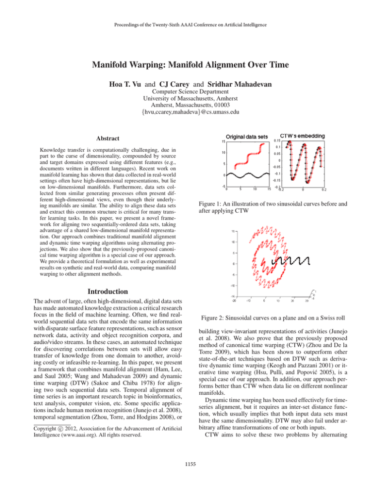
Figure 1: An illustration of two sinusoidal curves before and
after applying CTW
Introduction
The advent of large, often high-dimensional, digital data sets
has made automated knowledge extraction a critical research
focus in the field of machine learning. Often, we find realworld sequential data sets that encode the same information
with disparate surface feature representations, such as sensor
network data, activity and object recognition corpora, and
audio/video streams. In these cases, an automated technique
for discovering correlations between sets will allow easy
transfer of knowledge from one domain to another, avoiding costly or infeasible re-learning. In this paper, we present
a framework that combines manifold alignment (Ham, Lee,
and Saul 2005; Wang and Mahadevan 2009) and dynamic
time warping (DTW) (Sakoe and Chiba 1978) for aligning two such sequential data sets. Temporal alignment of
time series is an important research topic in bioinformatics,
text analysis, computer vision, etc. Some specific applications include human motion recognition (Junejo et al. 2008),
temporal segmentation (Zhou, Torre, and Hodgins 2008), or
Figure 2: Sinusoidal curves on a plane and on a Swiss roll
building view-invariant representations of activities (Junejo
et al. 2008). We also prove that the previously proposed
method of canonical time warping (CTW) (Zhou and De la
Torre 2009), which has been shown to outperform other
state-of-the-art techniques based on DTW such as derivative dynamic time warping (Keogh and Pazzani 2001) or iterative time warping (Hsu, Pulli, and Popović 2005), is a
special case of our approach. In addition, our approach performs better than CTW when data lie on different nonlinear
manifolds.
Dynamic time warping has been used effectively for timeseries alignment, but it requires an inter-set distance function, which usually implies that both input data sets must
have the same dimensionality. DTW may also fail under arbitrary affine transformations of one or both inputs.
CTW aims to solve these two problems by alternating
c 2012, Association for the Advancement of Artificial
Copyright Intelligence (www.aaai.org). All rights reserved.
1155
matrix W :
between canonical correlation analysis (CCA) (Anderson
2003) and DTW until convergence, as illustrated in Figure 1.
In the case where inputs are of different dimensions, CTW
first projects both data sets into a shared space using principal component analysis (PCA) (Jolliffe 2002). The algorithm does not always converge to a global optimum, but
CTW still improves the performance of the alignment when
compared to applying DTW directly. However, CTW fails
when the two related data sets require nonlinear transformations to uncover the shared manifold space. We illustrate
such a case in Figure 2, in which two sequential data sets are
two sin(x) curves; one lying on a plane and the other on a
Swiss roll. In this case, the CCA projection that CTW relies
on will fail to unroll the second curve, making a good DTW
alignment impossible.
We first provide a brief overview of manifold alignment
and dynamic time warping before combining the two to formulate manifold warping.
W =
k
=
− Fj
(X) 2
(X)
X
(Y )
− Fj
||Fi
(Y ) 2
F
(Y )
T
F·,k
LF·,k = 2tr F T LF
(4)
F
This matches the optimization problem of Laplacian
Eigenmaps (Belkin and Niyogi 2001), except that in this
case the similarity matrix is a joint matrix produced from
two similarity matrices. As with Laplacian Eigenmaps, we
add a constraint F T DF = I in order to remove an arbitrary scaling factor as well as to avoid a collapse to a subspace with dimension less than d. For example, this constraint prevents the trivial mapping to a single point. The
solution F = [f1 , f2 , ..., fd ] is given by d eigenvectors corresponding to the d smallest nonzero eigenvalues of the general eigenvalue problem: Lfi = λDfi for i = 1, ..., d.
We can also restrict the mapping to be linear by instead
solving the optimization problem:
argmin tr φT V T LV φ subject to φT V T DV φ = I
φ
(6)
, where V is the joint data set:
X 0
V =
(7)
0 Y
(X) φ
and φ =
is the joint projection, L, D are the graph
φ(Y )
Laplacian and degree matrix of V respectively. The resultant linear embedding is then Xφ(X) and Y φ(Y ) , instead
of F (X) and F (Y ) . The solution for φ = [φ1 , φ2 , ..., φd ]
is given by d eigenvectors corresponding to the d smallest nonzero eigenvalues of the general eigenvalue problem
V T LV φi = λV T DV φi for i = 0, ..., d.
|| Wi,j
|| Wi,j
2
X
||Fi,k − Fj,k ||2 Wi,j
i,j
, where L = D − W is the graph Laplacian of F , and D is
a diagonal matrix in which each diagonal element is the degree of the corresponding vertex. The optimization problem
becomes:
argmin (L1 ) = argmin tr F T LF
(5)
i,j∈X
+(1 − µ)
(3)
k
i∈X,j∈Y
(X)
XX
=
Suppose we have a mapping that maps X, Y to F (X) ∈
RnX ×d , F (Y ) ∈ RnY ×d in a latent space with dimension
d ≤ min(dx , dy ). Note that in terms of the underlying matrix representation, any row i of X is mapped to row i of
F (X) , and a similar relation holds for Y and F (Y ) . We form
the following loss function for the mapping as follows. The
first term indicates that corresponding points across data sets
should remain close to each other in the embedding. The last
two terms specify that, within an input set, points close in the
original space should remain close in the embedding. The
factor µ controls how much we want to preserve inter-set
correspondences versus local geometry.
X
(X)
(Y )
(X,Y )
L1 F (X) , F (Y ) = µ
||Fi − Fj ||2 Wi,j
||Fi
i,j
In manifold alignment (Wang and Mahadevan 2009), we are
given two data sets X ∈ RnX ×dX and Y ∈ RnY ×dY where
Rm×n denotes a m by n real matrix. In X and Y , each row
is an instance. W (X) ∈ RnX ×nX and W (Y ) ∈ RnY ×nY
are similarity matrices that provide the similarities between
instances in X and Y , respectively. These two matrices are
usually constructed as adjacency matrices of nearest neighbor graphs, optionally applying a heat kernel function. In addition, we also have a warping matrix W (X,Y ) ∈ RnX ×nY
that specifies the correspondences between instances in X
and Y. Typically,
1 if Xi corresponds to Yj
(X,Y )
Wi,j
=
(1)
0 otherwise
X
µW (X,Y )
(1 − µ)W (Y )
Then, we combine F (X) , F (Y ) into F where F =
F (X)
. Let Fi,k denote the element (i, k) of F and F·,k
F (Y )
denote the kth column of F . Then the loss function can be
rewritten:
X
L1 (F ) =
||Fi − Fj ||2 Wi,j
Manifold Alignment
+(1 − µ)
(1 − µ)W (X)
µW (Y,X)
(2)
i,j∈Y
Dynamic Time Warping
We are given two sequential data sets X = [xT1 , . . . , xTn ]T ∈
T T
Rn×d , Y = [y1T , . . . , ym
] ∈ Rm×d in the same space
with a distance function dist : X × Y → R. Let P =
The notation i ∈ X simply means 1 ≤ i ≤ nX . We can
combine W (X) ,W (Y ) , and W (X,Y ) into a joint similarity
1156
function for manifold warping:
L3 X
F (X) , F (Y ) , W (X,Y ) =
(X)
(Y )
(X,Y )
µ
kFi − Fj k2 Wi,j
i∈X,j∈Y
+(1 − µ)
+(1 − µ)
− Fj
(Y )
− Fj
kFi
(X) 2
(X)
(Y ) 2
(Y )
k Wi,j
(13)
k Wi,j
The optimization becomes
argmin
(L3 ) subject to
F (X) ,F (Y ) ,W (X,Y )
(X) F
F T DF = I where F =
and W (X,Y ) is a DTW
F (Y )
matrix. Note that unlike manifold alignment, the correspondence matrix W (X,Y ) is now an argument in the optimization problem. The intuition behind this loss function is similar to that of manifold alignment: the last two error terms
ensure that the embedding preserves the local geometry of
the inputs, and the first term promotes a high quality DTW
alignment between two sequential data sets. Again, these
goals are controlled by the parameter µ. We now propose
an algorithm that minimizes L3 :
{p1 , ..., ps } represent an alignment between X and Y , where
each pk = (i, j) is a pair of indices such that xi corresponds
with yj . Since the alignment is restricted to sequentiallyordered data, we impose the additional constraints:
= (1, 1)
= (n, m)
= (1, 0) or (0, 1) or (1, 1)
i,j∈X
X
(X)
kFi
i,j∈Y
Figure 3: A valid time-series alignment
p1
ps
pk+1 − pk
X
(8)
(9)
(10)
That is, an alignment must match the first and last instances and cannot skip any intermediate instance. This also
yields the property that no two sub-alignments cross each
other. Figure 3 is an example of a valid alignment. We can
also represent the alignment in matrix form W where:
1 if (i, j) ∈ P
Wi,j =
(11)
0 otherwise
Input: X,Y: two time-series data sets
d: latent space dimension
k: number of nearest neighbors used
µ: preserving correspondence vs local geometry factor
Output: F (X) , F (Y ) : the embeddings of X and Y in
the latent space
W (X,Y ) : the result DTW matrix that provides the
alignment of X and Y
begin
W (X) ← KNNGraph(X, k)
W (Y ) ← KNNGraph(Y, k)
(X,Y )
(X,Y )
Set W1,1
= WnX ,nY = 1, and 0 everywhere else
t←0
repeat (1 − µ)W (X)
µW (X,Y ),t
W =
µ(W (X,Y ),t )T (1 − µ)W (Y )
F (X),t+1 , F (Y ),t+1 ←
MA(F (X),t , F (Y ),t , W, d, µ)
W (X,Y ),t+1 ← DTW(F (X),t+1 , F (Y ),t+1 )
t←t+1
until convergence;
F (X) ← F (X),t ; F (Y ) ← F (Y ),t ;
W (X,Y ) ← W (X,Y ),t
end
To ensure that W represents an alignment which satisfies
the constraints in Equations 8, 9, 10, W must be in the following form: W1,1 = 1, Wn,m = 1, none of the columns
or rows of W is a 0 vector, and there must not be any 0 between any two 1’s in a row or column of W . We call a W
which satifies these conditions a DTW matrix. An optimal
alignment is the one which minimizes the loss function with
respect to the DTW matrix W :
X
L2 (W ) =
dist (xi , yj ) Wi,j
(12)
i,j
A naı̈ve search over the space of all valid alignments
would take exponential time; however, dynamic programming can produce an optimal alignment in O(nm).
Manifold Warping
One-step algorithm
We now present a novel framework for aligning two
sequentially-ordered data sets that share a common manifold representation. In our approach, we use the warping matrix produced by DTW as a heuristic correspondence matrix
for manifold alignment. The proposed algorithm uses alternating projections, picking new correspondences with DTW
and reprojecting both inputs using manifold alignment until
the loss function is minimized. This presents an improvement over CTW in cases where nonlinear transformations
are required to recover the underlying manifold structure of
one or both input data sets. We introduce the following loss
Algorithm 1: One-Step Manifold Warping
In Algorithm 1, MA(X,Y,W,d,µ) is a function that returns the embedding of X, Y in a d dimensional space using manifold alignment with the joint similarity matrix W
and parameter µ described in the manifold alignment section. The function DTW(X,Y) returns a DTW matrix after
aligning two sequences X, Y using dynamic time warping.
1157
The KNNGraph(X,k) function returns the k-nearest neighbors graph of a data set X. In some cases, it is useful to
replace the k-nearest neighbor graph approach with an neighborhood graph (Belkin and Niyogi 2001).
Theorem 1. Let L3,t be the loss function L3 evaluated at
F (X),t , F (Y ),t , W (X,Y ),t of Algorithm 1. The sequence L3,t
converges to a mimimum as t → ∞. Therefore, Algorithm 1
will terminate.
Input: X,Y: two time-series data sets
d: latent space dimension
k: number of nearest neighbors used
µ: preserving correspondence/local geometry factor
Output: F (X) , F (Y ) : the embeddings of X and Y in
the latent space
W (X,Y ) : the result DTW matrix that provides the
alignment of X and Y
begin
W (X) ← KNNGraph(X,k)
W (Y ) ← KNNGraph(Y,k)
t←0
F (X),t ← DimReduction F (X) , W (X) , d
F (Y ),t ← DimReduction F (Y ) , W (Y ) , d
repeat (1 − µ)W (X)
µW (X,Y ),t
W =
µ(W (X,Y ),t )T (1 − µ)W (Y )
(Y ),t+1
φ
, φ(X),t+1
← LMA F (X),t , F (Y ),t , W, d, µ
F (X),t+1 ← F (X),t φ(X),t+1
F (Y ),t+1 ← F (Y ),t φ(Y ),t+1
W (X,Y ),t+1 ← DTW F (X),t+1 , F (Y ),t+1
t←t+1
until convergence;
F (X) ← F (X),t ; F (Y ) ← F (Y ),t ;
W (X,Y ) ← W (X,Y ),t
end
Proof. In every iteration t, two steps are performed: using manifold alignment to solve for new projections
F (X),t+1 , F (Y ),t+1 , and using DTW to change the correspondences to W (X,Y ),t+1 .
Recall that the loss function L1 is just L3 with fixed
W (X,Y ) . In the first step, with fixed W (X,Y ),t , Algorithm
1 solves for new projections F (X),t+1 , F (Y ),t+1 using manifold alignment. In manifold alignment section, we showed
that manifold alignment’s mappings minimize the loss function L3 when the correspondence matrix is fixed. Hence:
L3 (F (X),t+1 , F (Y ),t+1 , W (X,Y ),t )
≤ L3 (F (X),t , F (Y ),t , W (X,Y ),t )
(14)
In the second step, the projections are fixed as
F (X),t+1 , F (Y ),t+1 . Algorithm 1 changes the correspondence matrix from W (X,Y ),t to W (X,Y ),t+1 which does not
(X)
(Y )
affect last two terms in L3 . If we replace dist(Fi , Fj )
(X),t+1
(Y ),t+1
by µ||Fi
− Fj
||2 in the loss function L2 of
DTW, we recover the first term in L3 of manifold warping.
Since W (X,Y ),t+1 is produced by DTW, it will minimize
the first term of L3 . Therefore, we have:
X
(X),t+1
(Y ),t+1 2
(X,Y ),t+1
µ
||Fi
− Fj
|| Wi,j
i∈X,j∈Y
X
≤µ
(X),t+1
||Fi
(Y ),t+1 2
− Fj
(X,Y ),t
|| Wi,j
Algorithm 2: Two-Step Manifold Warping
will use Laplacian Eigenmaps to be consistent with manifold alignment even though other methods such as LLE
(Roweis and Saul 2000), Isomap (Tenenbaum, De Silva, and
Langford 2000), etc. could be applied. LMA(X,Y,W,d,µ) is a
function that performs linear manifold alignment described
above on X and Y with the joint similarity matrix W , the
target dimension d and returns the projection matrices φ(X)
and φ(Y ) . We can think of DimReduction as a preprocessing
step, then reformulate the loss function as:
(15)
i∈X,j∈Y
Changing the correspondence matrix does not affect the last
two terms of L3 , so:
L3 (F (X),t+1 , F (Y ),t+1 , W (X,Y ),t+1 )
≤ L3 (F (X),t+1 , F (Y ),t+1 , W (X,Y ),t )
≤ L3 (F (X),t , F (Y ),t , W (X,Y ),t ) from inequality 14
⇔ L3,t+1 ≤ L3,t
)
L4 (φ(X) , φ(YX
, W (X,Y ) )
(X)
(X)
(X)
= ((1 − µ)
||Fi φ(X) − Fj φ(X) ||2 Wi,j
(16)
Therefore, L3,t is a decreasing sequence. We also have
L3,t ≥ 0, so it is convergent. Therefore, Algorithm 1 will
eventually terminate.
+(1 − µ)
+µ
Two-step algorithm
i,j∈X
X
(Y )
(Y )
(Y )
||Fi φ(Y ) − Fj φ(Y ) ||2 Wi,j
X i,j∈Y (X)
(Y )
(X,Y )
||Fi φ(X) − Fj φ(Y ) ||2 Wi,j
)
i∈X,j∈Y
We now propose an algorithm that exploits the observation
that if the local geometries of the two data sets are roughly
the same, their similarity matrices will also be very similar to each other. (Wang and Mahadevan 2008) Thus, if we
first perform a nonlinear projection on each input set independently, the embeddings are likely to be linearly alignable
using either manifold warping or CTW.
In Algorithm 2, DimReduction(X, W, d) is a dimensionality reduction function which maps X with similarity matrix W to a lower dimensional space d. In this paper, we
(17)
which is the same loss function as in linear manifold alignment except that W (X,Y ) is now a variable. The two constraints are the constraint in Equation 6 of linear manifold
alignment, and W (X,Y ) must be a DTW matrix.
Theorem 2. Let L4,t be the loss function L4 evaluated at
Qt
Qt
(X),i
, i=1 φ(Y ),i , W (X,Y ),t of Algorithm 2. The sei=1 φ
quence L4,t converges to a mimimum as t → ∞. Therefore,
Algorithm 2 will terminate.
1158
Proof. The proof is similar to that of theorem 1. At any iteration t, Algorithm 2 first fixes the correspondence matrix
at W (X,Y ),t . Now let L04 be like L4 except that we replace
(X)
(Y )
(X),t
(Y ),t
Fi , Fi
by Fi
, Fi
and Algorithm 2 minimizes
L04 over φ(X),t+1 , φ(Y ),t+1 using linear manifold alignment.
Thus,
L04 (φ(X),t+1 , φ(Y ),t+1 , W (X,Y ),t )
≤ L04 (I, I, W (X,Y ),t )
Qt
Qt
= L4 ( i=1 φ(X),i , i=1 φ(Y ),i , W (X,Y ),t )
= L4,t
(18)
Qt
since F (X),t = F (X),0 i=1 φ(X),i and F (Y ),t =
Q
t
F (Y ),0 i=1 φ(X),i . We also have:
L04 (φ(X),t+1 , φ(Y ),t+1 , W (X,Y ),t )
Qt+1
Qt+1
= L4 ( i=1 φ(X),i , i=1 φ(Y ),i , W (X,Y ),t )
≤ L4,t
Figure 4: Embedding of two sin(x2 ) curves illustrated in
Figure 2 onto 2D.
(19)
Algorithm 2 then performs DTW to change W (X,Y ),t to
W (X,Y ),t+1 . Using the same argument as in the proof of
Theorem 1, we have:
Qt+1
Qt+1
L4 ( i=1 φ(X),i , i=1 φ(Y ),i , W (X,Y ),t+1 )
Qt+1 (X),i Qt+1 (Y ),i
≤ L4 ( i=1 φ
, i=1 φ
, W (X,Y ),t )
(20)
≤ L4,t
⇔ L4,t+1 ≤ L4,t .
Figure 5: Result warping path of each algorithm’s alignment
and the ground truth warping path for the two sine curves
illustrated in Figure 2
So, the convergence follows.
Furthermore, when we set µ = 1, the loss function L4
will become similar to that of CTW. We can also substitute
CTW in place of the loop in the algorithm.
COIL-100 data set
We also test these algorithms on a real-world vision data
set from the Columbia Object Image Library (COIL100)
(S. A. Nene 1996). The corpus consists of different series
of images taken of different objects on a rotating platform.
Each series has 72 images, each 128 × 128 pixels. We try
to align two series of images of two different objects, with
differences in shape and brightness producing very different
high-dimensional representations. To demonstrate our algorithm’s ability to work with data sets of different dimensionality, we compress one image series to a smaller resolution
(64 × 64 pixels). Additionally, some duplicate images are
added to each series, to ensure that the correct mapping is
not trivially one-to-one.
In both experiments, manifold warping methods achieve
alignments with a much smaller error than CTW. The depiction in Figure 7 provides an intuitive picture of the manifold
warping algorithm. In the first projection to two dimensions,
both image series are mapped to circles. The next several iterations rotate these circles to match the first and last points,
then the points in between. For the case of one-step Manifold Warping (where all mappings are nonlinear), we pick a
small µ to prioritize preserving local geometry of each series. This avoids over-fitting the embedding to a potentially
bad intermediate DTW correspondence.
Experimental Results
Synthetic data sets
We compare the performance of CTW and manifold warping by trying to align two sin(x2 ) curves: one is on the flat
plane, the another is projected onto the Swiss roll as illustrated in Figure 2. Some duplicate points are added along the
curves to create many-to-one correspondences in the alignment.
As shown in Figure 4, manifold warping produced similar
embeddings for two curves based on their local geometry
while CTW linearly collapsed the Swiss roll curve onto the
plane.
As a result, the warping path (that is, the alignment path)
produced by manifold warping stays closer to the true warping path than that produced by CTW. The error is calculated
by the area between the result path and the ground truth path
as suggested in (Zhou and De la Torre 2009). We also normalize the error by dividing by the whole plot area, nX ×nY .
The warping paths and the calculated errors, shown in
Figure 5 and Table 1, show that manifold warping yields a
smaller error than CTW.
1159
Figure 6: Samples from pairs of COIL-100 image series
Figure 8: Warping paths for dog/cat toy images
Figure 7: 2D embedding of dog/cat toy image series (Figure
6).
Figure 9: 2D embedding of cup image series (Figure 6).
We perform the experiment with two pairs of COIL image
series, illustrated in Figure 6.
problem computationally feasible, we subsampled the original data sets. Each manifold warping method performs better
than CTW, based on the results shown below in Figure 11,
Figure 12, and Table 1.
Kitchen data set
Our last experiment uses the kitchen data set (De la Torre et
al. 2008) from the CMU Quality of Life Grand Challenge,
which records human subjects cooking a variety of dishes.
Here, we attempt nonlinear alignments between the same
subject and task, across different sensors.
Our experiment considers two separate views of the
same moment in time, during which the subject prepares a
brownie and an egg. The two views are 9-dimensional inertial measurement unit (IMU) readings and 87-dimensional
motion capture suit coordinates (MOCAP). Aligning two
views of the same task provides a straightforward evaluation metric, because the time stamps on each reading
yield ground-truth correspondence information. To make the
Synthetic
1-step
MW
2-step
MW
2-step
MW
CTW
Cups
0.0768
Dog
+Cat
0.0447
0.0464
Kitchen
Brownie
0.0257
Kitchen
Egg
0.0267
0.0817
0.0282
0.0125
0.0396
0.0469
0.0652
0.0298
0.0143
0.0772
0.0479
0.2784
0.2656
0.1668
0.0966
0.0510
Discussion and Future Work
Due to the lack of a linearity constraint, manifold warping
consistently performs better than CTW when the inputs lie
on manifolds that are not accessible via linear transformations. Even in the linear case, the alignment quality of manifold warping is at just as good as CTW.
Importantly, this improved alignment quality does not impose significant runtime overhead. Both algorithms rely on
the same DTW step, and tuned implementations of manifold
alignment are comparable in runtime to the CCA step used
in CTW. We found that while each manifold warping iteration is marginally slower than a similar CTW iteration, manifold warping tends to converge with fewer steps. Speedups
may be possible by using a relaxed variation of DTW for the
first few iterations, and parallelizing the initial alignments of
the two-step algorithm.
Both the one-step and two-step manifold warping algorithms are natural extensions of canonical time warping on
manifolds, and the results presented in this paper indicate
that this added information has the potential to significantly
improve alignment quality.
Several variants of DTW and manifold alignment may
prove beneficial within the manifold warping framework.
Future work will explore multiscale and local alignment
Table 1: Alignment error across algorithms and data sets
1160
Figure 10: Warping paths for cup images
Figure 12: Result warping path of each algorithm’s alignment for the kitchen data set - brownie experiment
Hsu, E.; Pulli, K.; and Popović, J. 2005. Style translation for
human motion. In ACM Transactions on Graphics (TOG),
volume 24, 1082–1089. ACM.
Jolliffe, I. 2002. Principal component analysis. Springer
series in statistics. Springer-Verlag.
Junejo, I.; Dexter, E.; Laptev, I.; Pérez, P.; et al. 2008. Crossview action recognition from temporal self-similarities.
Keogh, E., and Pazzani, M. 2001. Derivative dynamic time
warping. In First SIAM international conference on data
mining, 5–7.
Roweis, S., and Saul, L. 2000. Nonlinear dimensionality
reduction by locally linear embedding. Science 290(2323–
232).
S. A. Nene, S. K. Nayar, H. M. 1996. Columbia object
image library (coil-100). Technical Report CUCS-006-96.
Sakoe, H., and Chiba, S. 1978. Dynamic programming algorithm optimization for spoken word recognition. Acoustics, Speech and Signal Processing, IEEE Transactions on
26(1):43–49.
Tenenbaum, J.; De Silva, V.; and Langford, J. 2000. A global
geometric framework for nonlinear dimensionality reduction. Science 290(5500):2319–2323.
Wang, C., and Mahadevan, S. 2008. Manifold alignment using procrustes analysis. In Proceedings of the 25th international conference on Machine learning, 1120–1127. ACM.
Wang, C., and Mahadevan, S. 2009. A general framework
for manifold alignment. In AAAI Fall Symposium on Manifold Learning and its Applications.
Zhou, F., and De la Torre, F. 2009. Canonical time warping for alignment of human behavior. Advances in Neural
Information Processing Systems (NIPS) 1–9.
Zhou, F.; Torre, F.; and Hodgins, J. 2008. Aligned cluster
analysis for temporal segmentation of human motion. In
Automatic Face & Gesture Recognition, 2008. FG’08. 8th
IEEE International Conference on, 1–7. IEEE.
Figure 11: The embeddings of two sensors measurements
series IMU and MOCAP for a kitchen task involving
brownie.
strategies, enabling broader applications for manifold warping.
Acknowledgements
This material is based upon work supported by the National
Science Foundation under Grant Nos. NSF CCF-1025120,
IIS-0534999, and IIS-0803288.
References
Anderson, T. 2003. An introduction to multivariate statistical analysis. Wiley series in probability and mathematical statistics. Probability and mathematical statistics. WileyInterscience.
Belkin, M., and Niyogi, P. 2001. Laplacian eigenmaps and
spectral techniques for embedding and clustering. Advances
in neural information processing systems 14:585–591.
De la Torre, F.; Hodgins, J.; Bargteil, A.; Martin, X.; Macey,
J.; Collado, A.; and Beltran, P. 2008. Guide to the
carnegie mellon university multimodal activity (cmu-mmac)
database.
Ham, J.; Lee, D.; and Saul, L. 2005. Semisupervised alignment of manifolds. In Proceedings of the Annual Conference
on Uncertainty in Artificial Intelligence, Z. Ghahramani and
R. Cowell, Eds, volume 10, 120–127.
1161
