Proceedings of the Twenty-Fifth AAAI Conference on Artificial Intelligence
Stopping Rules for Randomized Greedy Triangulation Schemes
Andrew E. Gelfand, Kalev Kask and Rina Dechter
Bren School of Informatics and Computer Science
University of California, Irvine
Irvine, CA 92697, USA
stochastic algorithm be allowed to execute before performing inference on the best decomposition found so far?
Since query complexity is exponentially related to the induced width, investing the time to search for improved tree
decompositions may lead to a drastic reduction in the runtime of an inference procedure. We refer to the dilemma of
how long to seek good decompositions for as the Stopping
Problem because of its similarity to the problem of deciding when to stop software testing (Ross 1985). The stopping
problem is important when minimizing the time to respond
to a query. It is also important when a query must be answered within a certain amount of time, as the portion of
time spent seeking good decompositions can affect response
accuracy as well.
In this paper, we formalize the stopping problem in terms
of the total time needed to answer a probabilistic query. Doing so requires characterizing the run-time behavior of an
inference procedure that includes a stochastic component a difficult task because of the algorithm’s inherent randomness. Hoos and Stutzle analyzed the behavior of WalkSAT,
a stochastic local search algorithm for propositional satisfiability (SAT) problems, and empirically found it’s run-time
to be exponentially distributed(1999). Their analysis characterized the time WalkSAT requires to find a solution on a
random set of 3-SAT instances.
In this paper, we present an approach for estimating the
total run-time of an inference procedure that is instancespecific. We then propose a stopping rule that specifies when
to terminate execution of the stochastic component of the inference procedure. Fishelson and Geiger suggest terminating the stochastic component when the rate of occurrence
of improved tree decompositions falls below a threshold
(2003). In practice, several ad hoc rules are used to discontinue the search for improved tree decompositions. Notably,
the winning solver in two of the three tasks at the UAI 2010
approximate inference competition ran a stochastic variant
min-fill a fixed number of times on every problem instance1 .
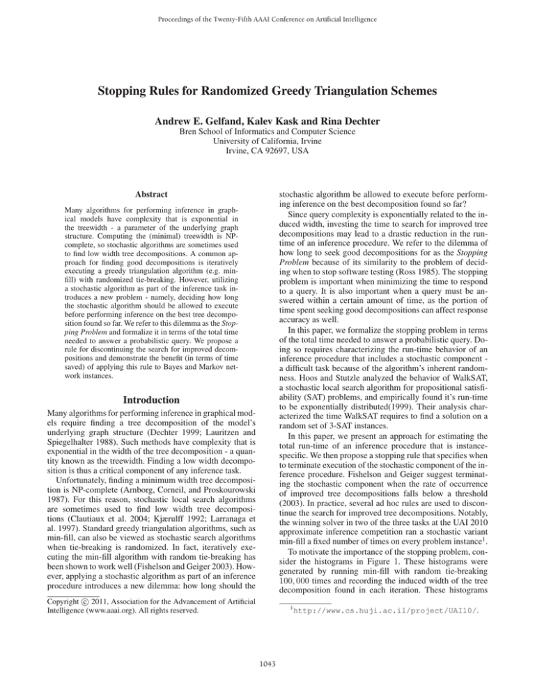
To motivate the importance of the stopping problem, consider the histograms in Figure 1. These histograms were
generated by running min-fill with random tie-breaking
100, 000 times and recording the induced width of the tree
decomposition found in each iteration. These histograms
Abstract
Many algorithms for performing inference in graphical models have complexity that is exponential in
the treewidth - a parameter of the underlying graph
structure. Computing the (minimal) treewidth is NPcomplete, so stochastic algorithms are sometimes used
to find low width tree decompositions. A common approach for finding good decompositions is iteratively
executing a greedy triangulation algorithm (e.g. minfill) with randomized tie-breaking. However, utilizing
a stochastic algorithm as part of the inference task introduces a new problem - namely, deciding how long
the stochastic algorithm should be allowed to execute
before performing inference on the best tree decomposition found so far. We refer to this dilemma as the Stopping Problem and formalize it in terms of the total time
needed to answer a probabilistic query. We propose a
rule for discontinuing the search for improved decompositions and demonstrate the benefit (in terms of time
saved) of applying this rule to Bayes and Markov network instances.
Introduction
Many algorithms for performing inference in graphical models require finding a tree decomposition of the model’s
underlying graph structure (Dechter 1999; Lauritzen and
Spiegelhalter 1988). Such methods have complexity that is
exponential in the width of the tree decomposition - a quantity known as the treewidth. Finding a low width decomposition is thus a critical component of any inference task.
Unfortunately, finding a minimum width tree decomposition is NP-complete (Arnborg, Corneil, and Proskourowski
1987). For this reason, stochastic local search algorithms
are sometimes used to find low width tree decompositions (Clautiaux et al. 2004; Kjærulff 1992; Larranaga et
al. 1997). Standard greedy triangulation algorithms, such as
min-fill, can also be viewed as stochastic search algorithms
when tie-breaking is randomized. In fact, iteratively executing the min-fill algorithm with random tie-breaking has
been shown to work well (Fishelson and Geiger 2003). However, applying a stochastic algorithm as part of an inference
procedure introduces a new dilemma: how long should the
c 2011, Association for the Advancement of Artificial
Copyright Intelligence (www.aaai.org). All rights reserved.
1
1043
http://www.cs.huji.ac.il/project/UAI10/.
Background
represent the typical variability in induced width observed
from running min-fill on linkage analysis instances2 . The
two empirical distributions in Figure 1 have very different shapes. The distribution of instance pedigree41 is more
heavily tailed than that of instance largeFam3-haplo-10-56.
This suggests that stochastic search will be more likely to
find a low width tree decomposition on largeFam3-haplo10-56 than on pedigree41. As such, more time should be invested seeking low width decompositions on instance pedigree41. The stopping problem involves deciding how much
time to invest on a new instance, with unknown distribution.
This section contains some necessary definitions.
D EFINITION 1. Graphical Model - A Graphical model R is
a 4-tuple R = X, D, F, ⊗, where:
1. X = {X1 , ..., Xn } is a set of variables;
2. D = {D1 , ..., Dn } is the respective set of finite domains;
3. F = {f1 , ..., fr } is a set of real-valued functions defined
over a subset of variables Si ⊆ X. The scope of function
fi , denoted scope(fi ), is its set of arguments, Si ;
4. ⊗i fi ∈ { i fi , i fi , i fi } is a combination operator.
A graphical model is the combination of functions: ⊗ri=1 fi .
Let G(X, E) denote an undirected graph, where X is the
set of nodes in the graph and E is the set of edges in the
graph. The primal graph G of a graphical model associates a
node with each variable and connects any two nodes whose
variables appear in the same scope. All the graphs considered in this paper are undirected and simple. Let nG (X)
denote the set of nodes that are neighbors of X in G and
ñG (X) the neighbors of X including X. A clique of G is a
set of nodes in G such that all the nodes are neighbors.
Eliminating a node X from G is a process resulting in the
creation of another graph G by: 1) adding (fill-in) edges to
make nG (X) a clique; and 2) removing X and its incident
edges from G. The number of fill-in edges needed to make
nG (X) a clique is the fill-in elimination cost of node X.
D EFINITION 2. Elimination Order - An elimination order
π is a total ordering of the nodes of G. π induces a sequence of graphs G1 = G, G2 , ...Gn , where Gi+1 is obtained from graph Gi by eliminating node π(i), the ith node
in the elimination order. π also induces a sequence of cliques
C1 , ..., Cn where Ci is the clique consisting of ñG (π(i)).
A tree decomposition can be constructed from an elimination order by connecting the cliques C1 , ..., Cn so as to
satisfy the running intersection property (see e.g. (Bodlaender and Koster 2010) for details).
D EFINITION 3. Induced Width - The induced width of elimination order π wrt graph G is
Histogram of induced widths for instance pedigree41
0.12
Normalized Frequency
0.1
0.08
0.06
0.04
0.02
0
25
30
35
40
45
50
Induced Width
55
60
65
(a) Pedigree41 (1062 variables))
Histogram of induced widths for instance largeFam3haplo1056
0.16
0.14
Normalized Frequency
0.12
0.1
0.08
0.06
0.04
0.02
0
45
50
55
60
65
70
Induced Width
75
80
85
(b) largeFam3-haplo-10-56 (2297 variables)
w(π, G) ≡ max |Ci | − 1
i=1...n
Figure 1: Histograms of induced widths from 100K iterations of min-fill with random tie-breaking.
(1)
The treewidth is the minimum induced width ordering across
all permutations of the nodes in G.
D EFINITION 4. Total State Space - The total state space of
an elimination order π wrt a graphical model R is:
The main contribution of this paper is to formulate
the Stopping Problem and formalize the trade-off between
searching for improved tree decompositions using a stochastic greedy triangulation algorithm and exploiting the best
decomposition found so far. The Stopping Problem is presented in Section 3, along with a novel Stopping Rule the Minimum Total Query Time (MTQT) rule. The fourth
section contains an empirical evaluation of the MTQT stopping rule and typical ad hoc stopping rules. The evaluation
demonstrates the benefit, in terms of time saved, of applying
the MTQT rule.
s(π, R) =
n
i=1
s(π(i), Gi )
(2)
where s(π(i), Gi ) = X∈ñG (π(i)) |DX | is the space rei
quired to eliminate node i from graph Gi and DX is the
domain of node X (Kjærulff 1992).
The min-fill heuristic is a greedy algorithm for constructing elimination orders. It operates as follows. Select the node
x whose elimination requires adding the fewest number of
edges (i.e. is of minimum fill-in elimination cost). Place this
2
Empirical distributions of more problems can be found at
http://www.ics.uci.edu/˜agelfand/elim.html.
1044
node in π(1) and eliminate it from the graph. Select a remaining node with minimum fill-in elimination cost, place it
in the next position in the order and eliminate it. Repeat until all nodes have been eliminated. More than one node may
have the minimum fill-in elimination cost in each step. The
stochastic min-fill algorithm breaks such ties by randomly
selecting from the set of minimum cost nodes.
The fill-in elimination cost is just one criteria for selecting the node eliminated in each step. Schemes that greedily
build elimination orders using other criterion were studied
in (Kjærulff 1992; Bodlaender and Koster 2010) and more
recently in (Kask et al. 2011).
it is plausible to express the total query time as
Tq (w) = Ts (w) + Tc (w)
where w ≡ w(π, G) is the induced width of ordering π in
the primal graph G of instance R. By making this simplification, we assume that all orderings of induced width w
have the same computation time. The ramifications of this
assumption are discussed in a following section.
Let ti ≥ 0 be the time that iteration i of the SOH completes. We model each completion of the SOH as an event
in a Poisson process whose rate is λ.3 Let wi be the induced width of elimination order πi . Let W be the set of
feasible4 widths and let W (j) denote the j th element in W
(|W
m| = m). Let πi be of width W (j) with probability pj
( j=1 pj = 1). If wi is independent of the previous orderings found, then each width W (j) will occur as an independent Poisson process with rate λj = λpj (Ross 2006). The
mean arrival time of an ordering of width W (j) is:
The Stopping Problem
In this section we formulate the stopping problem. Let
Tc (π, R) denote the time needed to compute a quantity (e.g.
a posterior marginal) in a Bayes or Markov network instance
R using elimination order π. We assume that the computation time is a deterministic quantity that depends on the
inference algorithm used. For example, in the experiments
section Tc is taken with respect to the Bucket Elimination
(BE) algorithm, whose performance is typical of most exact
inference algorithms (Dechter 1999).
Ultimately our goal is to minimize Tc . Since searching
over all possible orderings is infeasible, we utilize a stochastic ordering heuristic (SOH), such as min-fill with random
tie-breaking, to search for small computation cost elimination orders.
Executing a SOH for a period of time may yield improved
elimination orders. However, the time needed to find an improved ordering is uncertain. Let Ts (π, R) be a random variable describing the amount of time the SOH will take to find
ordering π. The total time to answer a probabilistic query,
Tq is the sum of the random variable Ts (π, R) and the deterministic quantity Tc (π, R). Tq is thus a random variable
expressed as:
Tq (π, R) = Ts (π, R) + Tc (π, R)
E [Ts (W (j))] = 1/λj = 1/(pj · λ)
i
π
(6)
λ and p = p1 , ..., pm are unknown and must be estimated.
The Maximum Likelihood estimate for the rate of a Poisson process when n events are observed by time tn is:
λ̂n = n/tn .
(7)
Let Xjn be the number of times an ordering of width W (j)
was observed in n iterations of the SOH. Then the vector
n
(X1n , ..., Xm
) follows a Multinomial distribution with parameters n,p. The posterior mean of pj at iteration n is:
X n + αj
j
(8)
p̂j,n = E pj |w(n) =
n + α0
of a Dirichlet prior
where αj are the parameters
m
Dir(α1 , ..., αm ) and α0 = j=1 αj .
The predicted total query time for a width W (j) ordering
given i iterations of the SOH is:
(3)
E[Tq (W (j))|w(i) , ti ] = E[Ts (W (j))]+Tc (W (j)) (9)
D EFINITION 5. Stopping Problem - Assume that we execute a SOH iteratively. Let ti denote the time that iteration i of the SOH completes and let πi be the elimination
(i)
(i)
order found in the ith iteration. Let Tq = ti + Tc denote the minimum total query time through iteration i, where
(i)
Tc = minij=1 Tc (πj , R) is the minimum computation time
through iteration i. The stopping problem is to identify the
index istop such that
Tq(istop ) = min Tq(i) = min Tq (π, R)
(5)
= 1/(λ̂i · p̂j,i ) + Tc (W (j))(10)
where w(i) = {w1 , ..., wi } and Tc is assumed to be known.
The MTQT stopping rule is described in the algorithm on
the following page.
Minimum Improvement (MI) Rule
The Minimum Improvement (MI) stopping rule is the procedure proposed in (Fishelson and Geiger 2003). This approach monitors the elimination orders found by the SOH
and terminates when the occurrence of improved orderings
becomes too infrequent.
(4)
We now present three rules for identifying istop .
Min Total Query Time (MTQT) Stopping Rule
3
The hypothesis that iterations of the SOH complete occur as
events of a Poisson process was empirically justified by fitting
an exponential distribution to the SOH execution times in several
problem instances.
4
W = {lb, ..., ub} is found by computing a lower bound lb using the minor-min-width heuristic and an upper bound ub by running the min-fill heuristic once prior to iteratively running the SOH.
The Minimum Total Query Time (MTQT) stopping
rule operates by making an estimate of the expectation
E[Ts (π, R)]. Combining this estimate with Tc (π, R) leads
to a stopping rule based on the expected total query time.
Since many inference algorithms have complexity that is
captured well by the induced width of an elimination order,
1045
The MTQT Stopping Rule
Input: Graphical Model R, feasible widths W and Dirichlet
prior parameters α1 , ..., αm
Output: stopping index istop
(0)
Initialization: Tc = ∞, done = false, i = 1
while done == false do
(πi , ti ) = SOH()
(i−1)
then
if Tc (πi , R) < Tc
(i)
Tc = Tc (πi , R)
end if
Update λ̂ with Eqn.7
done = true
for j = 1 to m do
Update p̂j with Eqn.8
(i)
if Tc (W (j)) + (λ̂ · pˆj )−1 < Tq then
done = false
end if
end for
i=i+1
end while
istop = i
model follows from the computational complexity of the BE
algorithm (Dechter 1999).
The model was fit as follows. First, we recorded the actual
run-time of BE on 1000 different elimination orders from
a small set of Markov network instances. These run-times
were treated as observations and âi ’s were found by minimizing the sum of squared error.
Tc (s), the computation time given the total state space of
an ordering (see Definition 4) was approximated in a similar
fashion using the model:
Tc (s) = a0 + a1 · s
(13)
This model does not contain instance specific parameters.
Experimental Results
This section contains an empirical evaluation of the proposed stopping rules. We describe the experimental setup,
the evaluation methodology and then discuss results.
Experimental Setup
This procedure utilizes the following ad hoc rule for terminating the SOH: if it took i iterations to find the current
best elimination order, allow an additional a × i iterations
to find a better ordering. The procedure is governed by two
parameters - a and b. a is a positive multiplication factor and
b > 0 is an integer threshold value that specifies the minimum number of times the SOH will be run.
We ran two sets of experiments to evaluate the stopping
rules. In the first set, query times were expressed using induced width - i.e. Tq (w(π, R)). In the second set, they were
expressed using total state space - i.e. Tq (s(π, R)).
The experiments were run on the set of Bayes and Markov
network instances shown in Table 1. Instances from the pedigree and mastermind problem classes were used in the solver
competition held at the UAI-2008 conference. Instances in
the largeFam3 problem class are derived from genetics. The
third column of Table 1 contains the average number of variables in each problem class. The fourth column contains the
average domain size, which may be less than 2 due to evidence. Standard deviations are shown in parentheses.
The parameters of each stopping rule were chosen via
10-fold cross-validation within each problem class. In the
MTQT procedure, we assumed each of the W possible
widths were equally likely - i.e. α1 = · · · = αm = α in
the Dirichlet prior. The value of β in the MI rule was set
in the range 1e−4 , ..., 1e−8 . The parameters of the MinMult
rule were chosen by considering all pairs (a b), where a ∈
A = {1...5} and b ∈ B = {100, 500, 1000, 5000, 10000}.
The evaluation also includes a baseline stopping rule in
which the min-fill algorithm is terminated after a fixed number of iterations. For the fixed rule, istop was chosen from:
100, 500, 1000, 5000, 10000, 50000.
Approximating Tc (w) and Tc (s)
Evaluation Methodology
The MI procedure operates as follows. The min-fill algorithm is run once to establish a baseline computation time
on the problem instance. The SOH is then run iteratively
and the improvement with respect to the baseline ordering
- the improvement ratio - is computed after each iteration.
The SOH is terminated when this ratio falls below some
threshold (β) or a maximum number of iterations has been
reached. In terms of total query time, the MI rule stops the
SOH at the first iteration istop in which:
(i
)
(i
)
+ Tc stop
ti
Tq stop
= stop
≤β
Tq (π1 , R)
t1 + Tc (π1 , R)
(11)
MinMult Rule
In formulating the stopping problem, we assume that
Tc (π, R) is a known deterministic quantity. In the MTQT
section, we proposed to express Tc as a function of w. Since
orderings with the same induced width may have different
computation times, this simplification prevents us from precisely computing Tc for a given ordering. As a result, we
approximate Tc (w) by a model of the following form:
(a +a2 ·w)
Tc (w) = a0 · nR · kR 1
The stopping rules were evaluated as follows. The min-fill
algorithm with random tie-breaking was run N = 100, 000
(12)
where nR is the number of variables in instance R, kR is the
average domain size and the ai ’s are model parameters. This
Problem Class # Inst. n̄
¯
|D|
pedigree
largeFam3
mastermind
2.0 (0.15)
1.54 (0.06)
2.0 (0.0)
22
122
128
917.1 (315.5)
3513.4 (806.6)
2158.8 (762.9)
Table 1: Summary of problem instances used in the experimental evaluation.
1046
Sample Total Query Time Computations
(i
)
(i )
Instance
istop log(Tq stop ) i
log(Tq )
pedigree18
70 7.32
102 6.54
pedigree34 26494 13.58
39490 12.09
pedigree7 27851 13.54
4239 13.53
times on each problem instance to generate a sequence of
induced widths w1 , ..., wN and state space sizes s1 , ..., sN .
The times that each min-fill iteration completed t1 , ..., tN
were also recorded. Given this sequence of observations, we
determined istop using each of the stopping rules. In practice, the stopping rules operate in an on-line fashion and do
not have access to all N observations. However, for evaluative purposes we require the full sequence of orderings.
We then identify the index i = arg minN
i=1 Tq (π(i) , R) at
which the total query time was minimized. i is found using
the estimates of Tc (w) (Tc (s)) described previously.
Figure 2 illustrates the difference between i and istop .
The figure contains a scatter plot of the induced widths
found in each iteration. The thick line traces the minimum width found through each iteration. The solid circle
at istop = 15296 indicates the stopping index predicted by
the MTQT rule. The solid square indicates the best possible
stopping iteration at i = 11090. Table 2 illustrates the total
query time computation on some pedigree instances.
Table 2: Total Query Time computations on selected pedigree instances (pedigree18 1184 variables; pedigree34 1160
vars; pedigree7 1068 vars).
Results
The results are organized into two different tables. Table
3 contains results from the experiments where Tq was expressed in terms of induced width and Table 4 contains the
total state space results. Each table is organized by problem class. The first row in each class, contains the parameter
settings of each stopping rule. The second and fourth rows
contain the seek time error and slow-down ratio of each stopping rule, averaged across the instances in a class. Standard
deviations are shown in parentheses.
The MTQT stopping rule performs quite well. In the total
state space experiments the MTQT rule had a smaller average SDR on all three problem classes. On the mastermind
instances, which have an average computation time of 640
hours5 , the difference between the SDR of the MTQT rule
(1.83) and the SDR of the MinMult rule (1.97) amounts to
an average savings of nearly 90 hours!
In the induced width experiments, the MTQT rule, fixed
rule and MinMult rule all yield comparable average SDR
on the pedigree and mastermind instances. The MTQT rule
yields the smallest average slow-down ratio on the largeFam3 instances, but does so by having a much larger, positive seek time error than the other methods. This suggests
that there is a natural trade-off between minimizing TErr
and SDR. On instances with large induced width (total state
space) TErr accounts for just a small portion of the total
query response time. Thus, if the goal is to minimize SDR,
it is generally better to overestimate the time at which the
minimum width (space) ordering will occur.
We close the experiments section by noting two ways in
which the performance of the MTQT procedure could be
improved. First, in our implementation of the MTQT rule
we assume that all widths in W , the set of feasible widths,
are equally likely to occur. In our experiments, the set W
was constructed by finding a lower and upper bound on the
induced width for a problem instance. As such, it is more
reasonable to assume a Dirichlet prior skewed towards the
upper bound. Second, approximating Tc (w) and Tc (s) in
the manner described is inherently inaccurate. Complexity
analysis of BE suggests the relationship between total state
space, induced width and computation time. However, the
run-time of BE cannot accurately be predicted as a function
of w or s alone. Identifying additional features of an ordering, or combining the features w and s into a single model
might improve BE run-time prediction accuracy.
Figure 2: Trace of the induced width of the elimination orders found by executing min-fill 100K times on instance
pedigree41. istop predicted by the MTQT rule is indicated
by the solid circle. i is indicated by a solid square.
The stopping rules were evaluated using two different
metrics. The first metric considered is the seek time error:
TErr = tistop − ti
(14)
which is the difference between the amount of time (in seconds) the SOH executed before being terminated by the
stopping rule and the amount of time the SOH needed to execute to find the minimum width (total state space) ordering.
The seek time error indicates how accurately the stopping
rule predicts the occurrence of the minimum width (total
state space) ordering. The sign of TErr provides an indication as to whether a stopping rule is under(over) estimating
the occurrence of the minimum width ordering. The second
metric considered is the slow-down ratio:
(istop)
SDR = Tq
/ Tq(i
)
(15)
This metric measures how much slower the total query response time is using a stopping rule than the smallest possible response time. The SDR measures how the choice of
stopping index impacts the total query response time.
5
This was computed using the average state space across all
mastermind instances.
1047
Class
Induced Width
MTQT MI
MinMult Fixed
pedigree
TErr
(TErr )
SDR
(SDR)
1e-4
24.7
(910.1)
2.29
(1.92)
1e-5
-118.7
(622.5)
4.11
(4.66)
5 1000
-154.2
(596.2)
2.99
(4.35)
10000
-104.8
(381.4)
2.17
(2.26)
largeFam3
TErr
(TErr )
SDR
(SDR)
1e-5
7572
(31513)
3.84
(4.03)
1e-5
-4695
(7746)
2.4e12
(2.6e13)
5 1000
-2498
(7546)
39.5
(250.2)
50000
3228
(6281)
8.67
(67.95)
mastermind
TErr
(TErr )
SDR
(SDR)
1e-3
15616
(35373)
1.89
(1.24)
1e-5
3493
(14032)
63.3
(164.3)
2 1000
-3928
(9303)
1.9
(1.06)
1000
-3972
(9276)
1.99
(1.52)
stantial. More analysis is needed to understand the graphical
model properties favorable for the MTQT rule.
This paper examined stopping rules to minimize the time
needed to exactly answer a probabilistic query. In many situations, a rapid approximate response is preferred to an exact
answer. This requires responding to a query within a certain amount of time (e.g. 20 seconds). The stopping problem becomes very important in such cases, as the portion
of time devoted to seeking good decompositions can affect
response accuracy as well. Much work remains to better understand the efficiency-accuracy tradeoff inherent to inference in graphical models. We see the stopping problem as
just one part of this important line of research.
Acknowledgments
This work was partially supported by NSF grants IIS0713118 and IIS-1065618 and NIH grant 5R01HG00417503. Thanks to the reviewers for their helpful feedback.
Table 3: Performance of the 4 stopping rules in the induced
width experiments. For each problem class we report: 1)
TErr averaged across the instances in the problem class;
and 2) the average SDR. Standard deviations are shown in
parentheses. TErr is reported in second. The parameter settings are listed in the first row of each problem class.
Class
Total State Space
MTQT MI
MinMult Fixed
pedigree
TErr
(TErr )
SDR
(SDR)
1e-2
556.4
(1046)
1.09
(0.16)
1e-7
259.9
(1037)
1.46
(1.38)
5 100
-363.7
(1047)
1.41
(0.55)
50000
182.3
(555.5)
1.14
(0.20)
largeFam3
TErr
(TErr )
SDR
(SDR)
1e-10
6961
(9249)
1.31
(0.79)
1e-8
7362
(9923)
1.2e9
(1.3e10)
5 5000
-894.5
(11406)
12.73
(52.31)
50000
-83.3
(5291)
2.69
(6.97)
mastermind
TErr
(TErr )
SDR
(SDR)
1e-3
-2209
(23577)
1.83
(0.85)
1e-5
-12621
(27361)
30.98
(68.7)
2 1000
-16447
(27545)
1.97
(1.55)
10000
-14450
(24526)
4.24
(6.61)
References
Arnborg, S.; Corneil, D.; and Proskourowski, A. 1987.
Complexity of finding embeddings in a k-tree. SIAM Journal of Discrete Mathematics. 8:277–284.
Bodlaender, H. L., and Koster, A. M. C. A. 2010. Treewidth
computations i: Upper bounds. Inf. Comput. 259–275.
Clautiaux, F.; Moukrim, A.; Negre, S.; and Carlier, J. 2004.
Heuristic and meta-heuristic methods for computing graph
treewidth. RAIRO Operations Research 38:13–26.
Dechter, R. 1999. Bucket elimination: A unifying framework for reasoning. Artificial Intelligence 113:41–85.
Fishelson, M., and Geiger, D. 2003. Optimizing exact genetic linkage computations. RECOMB 114–121.
Hoos, H., and Stutzle, T. 1999. Towards a characterization
of the behaviour of stochastic local search algorithms for sat.
Artificial Intelligence 112:213–232.
Kask, K.; Gelfand, A.; Otten, L.; and Dechter, R. 2011.
Pushing the power of stochastic greedy ordering schemes
for inference in graphical models. In AAAI 2011.
Kjærulff, U. 1992. Optimal decomposition of probabilistic
networks by simulated annealing. Statistics and Computing
2:2–17.
Larranaga, P.; Kuijpers, C.; Poza, M.; and Murga, R. 1997.
Decomposing bayesian networks: triangulation of the moral
graph with genetic algorithms. Statistics and Computing
7:19–34.
Lauritzen, S., and Spiegelhalter, D. 1988. Local computation with probabilities on graphical structures and their application to expert systems. Journal of the Royal Statistical
Society, Series B 50(2):157–224.
Ross, S. 1985. Software reliability: The stopping rule problem. IEEE Trans. on Software Engineering 11:1472–1476.
Ross, S. 2006. Introduction to Probability Models, Ninth
Edition. Orlando, FL, USA: Academic Press, Inc.
Table 4: Performance on the total state space experiments.
Conclusions
The main contribution of this paper was to formulate the
Stopping Problem. This allowed us to formalize the trade-off
between seeking improved elimination orders and exploiting
the best ordering found so far. We then presented three different Stopping Rules for identifying when to discontinue
the search for improved orderings and empirically evaluated
these rules on a set of Bayes and Markov network instances.
The empirical evaluation showed that the MTQT rule reliably leads to smaller total query response times than ad hoc
stopping rules that are used in practice. In many problems,
the time savings due to the MTQT stopping rule are sub-
1048