Proceedings of the Twenty-Fifth AAAI Conference on Artificial Intelligence
Multi-Task Learning in Square Integrable Space
Wei Wu
Hang Li, Yunhua Hu
Rong Jin
MOE-Microsoft Key Laboratory of Statistics
and Information Technology, Peking University
v-wew@microsoft.com
Microsoft Research Asia
hangli@microsoft.com
yuhu@microsoft.com
Computer Science and Engineering
Michigan State University
rongjin@cse.msu.edu
Abstract
ϱϬ
Several kernel based methods for multi-task learning have
been proposed, which leverage relations among tasks as regularization to enhance the overall learning accuracies. These
methods assume that the tasks share the same kernel, which
could limit their applications because in practice different
tasks may need different kernels. The main challenge of introducing multiple kernels into multiple tasks is that models
from different Reproducing Kernel Hilbert Spaces (RKHSs)
are not comparable, making it difficult to exploit relations
among tasks. This paper addresses the challenge by formalizing the problem in the Square Integrable Space (SIS). Specially, it proposes a kernel based method which makes use of
a regularization term defined in the SIS to represent task relations. We prove a new representer theorem for the proposed
approach in SIS. We further derive a practical method for
solving the learning problem and conduct consistency analysis of the method. We discuss the relations between our
method and an existing method. We also give an SVM based
implementation of our method for multi-label classification.
Experiments on two real-world data sets show that the proposed method performs better than the existing method.
ϯϬ
ϰϬ
ϮϬ
ϭϬ
ůĂƐƐϭ
ůĂƐƐϮ
Ϭ
ͲϳϬ
ͲϲϬ
ͲϱϬ
ͲϰϬ
ͲϯϬ
ͲϮϬ
ͲϭϬ
Ϭ
ϭϬ
ϮϬ
ϯϬ
ϰϬ
ͲϭϬ
ϱϬ
ϲϬ
ůĂƐƐϯ
ůĂƐƐϭΘϮ
ͲϮϬ
ͲϯϬ
ͲϰϬ
ͲϱϬ
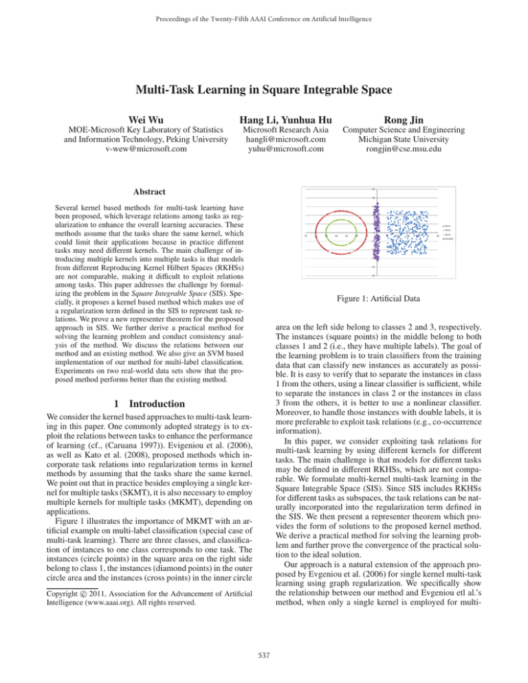
Figure 1: Artificial Data
area on the left side belong to classes 2 and 3, respectively.
The instances (square points) in the middle belong to both
classes 1 and 2 (i.e., they have multiple labels). The goal of
the learning problem is to train classifiers from the training
data that can classify new instances as accurately as possible. It is easy to verify that to separate the instances in class
1 from the others, using a linear classifier is sufficient, while
to separate the instances in class 2 or the instances in class
3 from the others, it is better to use a nonlinear classifier.
Moreover, to handle those instances with double labels, it is
more preferable to exploit task relations (e.g., co-occurrence
information).
In this paper, we consider exploiting task relations for
multi-task learning by using different kernels for different
tasks. The main challenge is that models for different tasks
may be defined in different RKHSs, which are not comparable. We formulate multi-kernel multi-task learning in the
Square Integrable Space (SIS). Since SIS includes RKHSs
for different tasks as subspaces, the task relations can be naturally incorporated into the regularization term defined in
the SIS. We then present a representer theorem which provides the form of solutions to the proposed kernel method.
We derive a practical method for solving the learning problem and further prove the convergence of the practical solution to the ideal solution.
Our approach is a natural extension of the approach proposed by Evgeniou et al. (2006) for single kernel multi-task
learning using graph regularization. We specifically show
the relationship between our method and Evgeniou etl al.’s
method, when only a single kernel is employed for multi-
1 Introduction
We consider the kernel based approaches to multi-task learning in this paper. One commonly adopted strategy is to exploit the relations between tasks to enhance the performance
of learning (cf., (Caruana 1997)). Evigeniou et al. (2006),
as well as Kato et al. (2008), proposed methods which incorporate task relations into regularization terms in kernel
methods by assuming that the tasks share the same kernel.
We point out that in practice besides employing a single kernel for multiple tasks (SKMT), it is also necessary to employ
multiple kernels for multiple tasks (MKMT), depending on
applications.
Figure 1 illustrates the importance of MKMT with an artificial example on multi-label classification (special case of
multi-task learning). There are three classes, and classification of instances to one class corresponds to one task. The
instances (circle points) in the square area on the right side
belong to class 1, the instances (diamond points) in the outer
circle area and the instances (cross points) in the inner circle
c 2011, Association for the Advancement of Artificial
Copyright Intelligence (www.aaai.org). All rights reserved.
537
ple tasks in our method. We give a specific algorithm of
our method based on SVM technique. Experiments of multilabel classification on two real-world data sets show that
our approach performs better than the existing method for
MKMT problems.
Our contribution in this paper is primarily theoretical, and
it consists of three fold: (1) proposal of a method of multitask learning in Square Integrable Space, particularly for
MKMT, (2) theoretical analysis of the method, (3) practical implementation of the method and empirical verification
of its effectiveness.
ploiting label correlation. They focus on learning of a better
feature representation by employing MKL, while we try to
solve a multi-task learning problem. Duan et al. (2009) proposed learning classifiers in different function spaces for different tasks in domain adaptation (similar to MKMT). They
trained classifiers separately, rather than collectively as in
multi-task learning.
3 Premise
In this section, we define notations used in this paper and
introduce some background knowledge.
2 Related Work
Notations
Multi-task learning aims to perform learning for multiple
problems simultaneously in order to achieve better performance for all the problems. It has been verified both theoretically and empirically that it is feasible if one can properly
leverage information across the tasks in the learning process, and many methods have been proposed (cf.,(Caruana
1997)). One group of methods attempt to use task relations.
For example, Evgeniou et al. (2006), and Kato et al.(2008)
proposed presenting task relations as regularization terms in
the objective functions to be optimized. The regularization
terms can make closer the parameters of models for similar
tasks. Another group of methods manage to find the common structure for multi-task learning. For instance, Ando
& Zhang (2005), as well as Argyriou et al. (2007) proposed methods for multi-task learning by finding the common structure from data, and then utilizing the learned structure. Our multi-task learning method belongs to the first
group, and it is more generally applicable than the existing
methods (MKMT v.s. SKMT).
Kernel methods are a principled and powerful approach
in machine learning (Schölkopf and Smola 2002). Conventional kernel methods are defined in the Reproducing Kernel
Hilbert Space (RKHS). In our paper, we extend kernel methods to the Square Integrable Space (SIS).
One issue in kernel methods is to choose a proper kernel from a set of candidate kernels. A common practice is
to heuristically determine a set of kernels, compare the performances of the kernels, and choose the best one. Multiple Kernel Learning (MKL) aims to solve the kernel selection problem in a principled way. Specifically, it employs a linear combination of kernels and learns the model
(classifier) as well as the optimal weights of the linear
combination at the same time (c.f., (Lanckriet et al. 2002;
Bach, Lanckriet, and Jordan 2004)). MKMT is different
from MKL; the former is about learning for multiple tasks,
while the latter is about kernel selection in a single task. We
could adopt MKL in selection of the best kernel for each
task (the best linear combination of kernels) in our method.
In this paper, we simply use the heuristic way of kernel selection and consider integration of MKL into our approach
as future work.
The following recent work is also related to, but different from our work. Tang et al. (2009) proposed a method of
simultaneously learning multiple kernels for multiple tasks,
but they did not utilize task relations. Ji et al. (2009) proposed to embed data into a low dimensional space by ex-
We consider multi-task learning, specifically, multi-label
learning. Suppose that there are T tasks. For each task t, data
(xt , yt ) is generated from Xt × Yt according to a distribution
Pt (x, y). In this paper, we consider multi-label classification.
We assume that Xt =X for all tasks and xt is independent
from t. X is a compact subset in Rd and Yt = {+1, −1}.
Moreover, we have a training data set S t = {(xi , yti )}ni=1 for
each task t and our goal is to learn a classifier ft (·): X → R
that can assign a label to a new instance x. Different tasks
share a common marginal distribution P(x) but have different conditional distributions Pt (y|x). In MKMT, the function
spaces Ft ( ft (·) ∈ Ft ) of different tasks are assumed to be
different.
We further assume a matrix Δ ∈ RT+×T is provided as prior
knowledge in training, where element δ(s, t) ∈ [0, 1] represents the similarity between tasks s and t. In this paper, we
give a heuristic way to learn Δ from training data for multilabel classification in Section 6. We use Δ in learning of the
classifiers { ft (·)}Tt=1 .
RKHS and Square Integrable Space
We briefly review the theory on Reproducing Kernel Hilbert
Space (RKHS) (Aronszajn 1950) and show the relationship
between RKHS and Square Integrable Space (SIS).
A Hilbert space H of functions f (·) : X → R is an RKHS
if and only if there is a function K(·, ·) : X×X → R that satisfies1) K(x, y) = K(y, x) ∀x, y ∈ X ; 2) ∀{αi }ni=1 ⊂ R, {xi }ni=1 ⊂
X, ni, j=1 αi α j K(xi , x j ) 0 such that f (x) = f (·), K(x, ·)H
∀x. K(·, ·) is called a reproducing kernel.
A continuous reproducing kernel K is a Mercer kernel.
Suppose that X is endowed with a measure μ, μ(X) < ∞.
We use L2 (X, μ) to denote square integrable
function space
of X in which each function f (·) satisfies f 2 (x)μ(dx) < ∞.
According to Mercer Theorem (Cucker and Smale 2002),
2
there is an orthonormal
basis {ei (·)} of L (X, μ) associated
with K and K(x, y) = i λi ei (x)ei (y) ∀x, y ∈ X. ∀i, λi 0 is
the i-th eigenvalue and ei (·) is continuous.
The following theorem (Cucker and Smale 2002) unveils
that for any Mercer kernel K, the RKHS HK is a subspace
of Square Integrable Space.
Theorem 3.1. HK = { f ∈ L2 (X, μ)| f (·) = ∞
i=1 ai ei (·),
∞ a2i
∞ a2i
2
i=1 λi < ∞}. ∀ f ∈ HK , || f ||HK =
i=1 λi , and f is continuous on X.
538
4 Our Approach
problem (1) becomes
We propose a novel and general kernel approach to multitask learning using task relations. Formally, suppose that
RKHS Ht is generated by kernel κt for task t. We learn function (model) ft from Ht . Since kernels κt may be different from each other, f1 , f2 , . . . , fT may be no longer in the
same space (i.e., RKHS). We consider using Square Integrable Space (SIS) as the space containing all the RKHSs
Ht , which is supported by Theorem 3.1. We conduct multitask learning in L2 (X, P(x)), where P(x) is the marginal distribution on X (We specifically let μ in Theorem 3.1 be P(x)
in this paper).
One advantage of the approach is that we can naturally use
task relations in L2 (X, P(x)), since SIS contains the RKHSs
for different tasks. More importantly, we can offer a theoretical justification to the approach by proving the representer
theorem and the convergence of the practical solution.
fˆt (·) =
T
Convergence of Practical Solution
In this section, we further assume that L is differentiable and
prove the convergence of practical solution under the condition 2 . Theorem 4.5 gives a bound on the difference between
the two solutions. The result indicates that the practical solution (3) converges to the ideal solution (2) in probability.
We briefly explain how to obtain the bound and present the
proof of Theorem 4.5 in Appendix B.
Define Dt = sup x∈X | ft (x) − fˆt (x)|. Suppose that
max1tT sup x∈X κt (x, x) B. Define h(F , X) =
sup f ∈F |E f 2 − n1 ni=1 f 2 (xi )|, where X = {xi }ni=1 , F = { f | f =
T
ft , ft ∈ Ht , ft κt R∗ }. Since { ft (·)}Tt=1 minimize (1),
t=1
T
1 T n
TU
2
t=1 || ft ||κt nγ1
t=1 i=1 L(0, yti ) γ1 , where L(0, y) T
U. Similarly, t=1 || fˆt ||2κt TγU1 . We can let R∗ = TγU1 , thus,
∀t, s, ft − f s and fˆt − fˆs are in F . We first bound h(F , X).
Using the McDiarmid inequality (Bartlett and Mendelson
2002), we obtain the following lemma:
ft ∈Ht
T
n
(1)
where the second term is a normal regularization term which
controls the complexity of models in their own RKHSs, and
the third term is a regularization term which measures difference of models in the common space (i.e.,L2 (X, P(x))). The
underlying assumption is that if two tasks s and t are similar
(δ(s, t) is large), then the corresponding models should also
be similar in the common space.
To guarantee the existence of solution and identify the
form of solution, we need a new Representer Theorem for
the new kernel method:
Lemma 4.2. Given an arbitrary small positive number δ,
with probability at least 1−δ, the following inequality holds:
2 ln(2/δ)
∗ 2
.
|h(F , X) − Eh(F , X)| (T R ) B
n
With this lemma, we only need to bound Eh(F , X). Using the conclusion (Theorem 12.6) and some proof techniques (proof of Theorem 8 and Lemma 22) in (Bartlett and
Mendelson 2002), we obtain
Theorem 4.1 (Representer Theorem). Suppose that loss
function L(·, ·) is non-negative, convex and continuous, the
solution to the optimization problem (1) exists and has the
following form:
ft (·) =
n
Lemma 4.3.
8(T R∗ )2 B
√
n
Combining the results in Lemma 4.2 and 4.3, we finally
obtain the bound for h(F , X):
E(h(F , X)) ≤
αti κt (xi , ·) +
θt (y)κt (y, ·)P(dy),
(2)
i=1
where αti ∈ R and θt (·) ∈ L2 (X, P(x)).
Formula (2) offers an ideal solution. The proof sketch of
Theorem 4.1 is given in Appendix A.
Theorem 4.4. With probability at least 1 − δ, we have the
following inequality hold:
2 ln(2/δ) 8(T R∗ )2 B
∗ 2
g(n).
+
h(F , X) ≤ (T R ) B
√
n
n
Practical Solution
To obtain the ideal solution, we need to know marginal
distribution P(x), and then solve a functional optimization
problem (Note θt is a L2 integrable function).
In practice, we use the empirical distribution P̂(x) =
1 n
1
to estimate P(x). Thus, the solution of
i=1 1(x = xi )
n
1
(3)
We need to answer the question whether the practical solution converges to the ideal solution when the training data
size goes to infinity. As shown below, we are able to prove
the convergence, by analyzing the relationship between the
two minimums of the optimization problem (1) under P(x)
and P̂(x) respectively.
Multi-task learning is then defined as the following optimization problem:
1 L( ft (xi ), yti ) + γ1
ft 2κt
n t=1 i=1
t=1
T
γ2
+
δ(s, t) ( f s (x) − ft (x))2 P(dx),
2 s,t=1
1
θti κt (xi , ·).
n i=1
n
αti κt (xi , ·) +
i=1
Ideal Solution
arg min
n
With the results above, we reach our conclusion:
2
Whether the same conclusion holds under a weaker condition
is still an open question, in which L is only continuous. Our hypothesis is that it may be the case, because we can use differentiable
functions to approximate a continuous function (e.g., Weierstrass
Approximation Theorem).
1(x = xi ) = 1, if x = xi , otherwise, 1(x = xi ) = 0
539
Theorem 4.5. With probability at least 1 − δ, the following
inequality holds:
Algorithm 1
1: Input: training data {xi }ni=1 ,{yti }ni=1 1 t T , task similarity
matrix Δ
2: Choose a proper kernel κt for each task t
3: Choose proper γ1 and γ2 .
4: Compute matrix (K + γγ2 K(L ⊗ I)K)−1
1
5: Compute β∗ by solving the dual problem
6: Compute α∗ by using equation (5).
∗
7: Output: ft∗ (·) = nt=1 α∗
ti κt (xi , ·) + bt , 1 t T
1
Dt = sup| ft (x) − fˆt (x)| O(1/n 4 ) 1 t T.
x∈X
Relation with Existing Approach
Evgeniou et al. (2006) exploit task relations (i.e. Δ) to conduct multi-task learning through the following optimization
problem :
1 L( ft (xi ), yti ) + γ1
|| ft ||2κ
n t=1 i=1
t=1
T
arg min
{ ft }⊂H
T
n
we obtain the dual problem:
(4)
arg max
T
γ2 +
δ(s, t)|| f s − ft ||2κ .
2 s,t=1
β∈RnT
α∗ =
5 Implementation
6
We give a specific algorithm of our approach. We define the
loss function L as hinge loss. Moreover, we also add a bias
bt into each classifier ft (·) following the convention. By introducing slack variables, we can obtain the primal problem:
ft ∈Ht
t=1 i=1
1
γ2
(K + K(L ⊗ I)K)−1 KYβ∗ .
2γ1
γ1
(5)
The details of the algorithm are shown in Algorithm 1. At
step 2, we empirically find a proper kernel for each task,
from a number of kernels. At step 5, we solve a QP problem. We specifically employ Franke and Wolf’s method (see
(Elisseeff and Weston 2002)), which is a gradient descent
based method. At step 4, we need to compute the inverse of
a matrix, which is of order O((T n)3 ). We focus on problem
formulation and theoretical analysis in this paper, and leave
to future work the improvements of our method on efficiency
and kernel selection.
The theorem indicates that for SKMT cases our approach
can work as well as existing approach.
T
0 βti 1.
Here, β = (β1 , β2 , . . . , βT ) is the dual variable where
βt = (βt1 , βt2 , . . . , βtn ) t = 1, 2 . . . T . Y is a diagonal matrix
whose t × i-th element is yti . L is the task graph Laplacian
which is constructed by taking δ(s, t) as the weight of edge
connecting task s and t on an undirected graph. I is an identity matrix. K is a block diagonal matrix with each block
Kt = (κt (xi , x j ))n×n .
After getting the optimal β∗ , we can compute the optimal α∗ = (α1 ∗ , α2 ∗ , . . . , αT ∗ ) where αt ∗ =
(αt1 ∗ , αt2 ∗ , . . . , αtn ∗ ) through the following equation:
where C(κ, P(x)) is a positive constant related to kernel κ
and the marginal distribution P(x). Moreover, if κ satisfies
κ(x, y) 0 and κ(x, y)P(dx) = 1 ∀y (e.g., Gaussian kernel), C(κ, P(x)) 1.
ξti + γ1
t=1 i=1
n
1 γ2
β YK(K + K(L ⊗ I)K)−1 KYβ
4γ1
γ1
i=1
Theorem 4.6. Suppose all tasks share the same kernel κ,
∀s, t, the following inequality holds:
2
δ(s, t)|| f s − ft ||κ C(κ, P(x))δ(s, t) ( f s (x) − ft (x))2 P(dx),
T n
βti −
βti yti = 0, 1 t T,
where the second term is a regularization term in RKHS, and
the third term is a regularization term based on task relations, also defined in the RKHS. In their approach , in order
to make comparison between models for different tasks and
exploit task relations, models are assumed to be in the RKHS
generated by the same kernel κ, which is the major difference
from our approach. Our approach (1) extends their approach
and can handle both SKMT and MKMT cases. When all
tasks share the same kernel, the following theorem shows
the relationship between the two regularization terms of our
approach and Evgeniou et al.’s approach:
arg min
T n
Experiments
We conducted experiments on multi-label classification to
verify the effectiveness of our approach. We used two realworld classification data sets: protein data and music data.
We considered two baselines: Individual and Single (Kernel). In the former, SVM classifiers for the tasks are trained
individually (i.e., task relations are ignored), and in the latter, SVM classifiers for tasks are trained using Evgeniou et
al.’s method (4). We denote our method Multiple (Kernel).
As evaluation measure, we utilized ROC score (Lanckriet et
al. 2004).
In our experiments, we employ the following heuristic
method to learn {δ(s, t)} from training data. We create a vector for each task (class) based on training data. Each element
of the vector corresponds to an instance; and if the instance
|| ft ||2κt
t=1
T
n
γ2 +
δ(s, t)( f s (xi ) − ft (xi ))2
2 s,t=1 i=1
yti ( ft (xi ) + bt ) 1 − ξti , ξti 0.
Combining αti and 1n θti in Equation (3) as αti and substituting
the solution given by Equation (3) into the primal problem,
540
belongs to the class (task), then we set the value of the element as 1, otherwise we set it as 0. Finally, we take the
cosine of the vectors of two tasks s and t as δ(s, t). We actually use co-occurrence of tasks (classes) as similarity between them.
Both of the two real-world data sets are on multi-label
classification. The first data set 3 is on classification of protein functions, which contains 3, 588 proteins with 13 function classes. The average number of functions per protein is
1.53. For more details about the data set, see (Lanckriet et
al. 2004). The second data set 4 is on music emotion classification, which contains 593 pieces of music and 6 types of
emotion. The average number of emotion types per piece of
music is 1.87.
we randomly chose 500 instances for protein data and 100
instances for music data as training data, respectively, and
evenly divided the rest into two subsets as validation and
testing data for both data sets. We used the heuristic method
to calculate task similarities from the training data.
For protein data, no information on features is available, and the kernels are provided as kernel matrices. There
are in total 8 kernel matrices (8 kernels). For music data,
2
we created Gaussian kernels (e−σ||x−y|| ) with σ varying in
{0.01, 0.05, 0.1, 0.5, 1, 5, 10}, linear kernel, and polynomial
kernels with degree 2 − 5 as kernel candidates. We chose γ1
from {0.1, 0.5, 1, 5}, and γ2 from {0.01, 0.05, 0.1, 0.5, 1, 5}.
Kernel selection and parameter tuning were conducted using the validation data. First, kernels were selected and parameter γ1 was tuned for Individual. Next, the kernels and
parameter γ1 were fixed, and parameter γ2 was tuned for
Multiple. Finally, the kernels of Individual were used, and
the two parameters of γ1 and γ2 were simultaneously tuned
for Single.
We repeated the above process ten times, and the final results are averaged over ten trials. Table 1 gives the results of
three methods on two data sets. On protein data, for classes
2, 8, 10, and 13 the best performing kernel for Individual is
Smith-Waterman kernel (K sw ), and for the other classes the
best performing kernel is Enriched Pfam kernel (K p f amE ).
Superscripts 1, 2, and 3 stand for that the improvements of
our methods are statistically significant over Individual, Single using kernel K sw and Single using kernel K p f amE , respectively. On music data, for classes except 3, polynomial kernel with degree 5 performs best, and for class 3, Gaussian
kernel with σ = 0.01 is the best performing one. Superscripts 1, 2, and 3 stand for that the improvements of our
methods are statistically significant over Individual, Single
using Gaussian kernel and Single using polynomial kernel,
respectively.
From the results in Table 1, we can see that kernel selection is crucial for Single. With a good kernel selection,
SKMT’s performance can be comparable to Multiple, but
with a bad kernel selection, the performance can be worse
than Individual. In contrast, Multiple can exploit different
kernels as well as the task relations to achieve an overall
good performance.
3
4
Table 1: Comparison of three methods on two real-world
data sets
class 1
class 2
class 3
class 4
class 5
class 6
class 7
class 8
class 9
class 10
class 11
class 12
class 13
Average
Comparison of three methods on protein data
Individual
Single (K sw )
Single (K p f amE )
0.721
0.697
0.736
0.666
0.652
0.638
0.654
0.655
0.653
0.728
0.745
0.741
0.779
0.790
0.779
0.682
0.650
0.686
0.671
0.653
0.673
0.635
0.641
0.621
0.605
0.584
0.611
0.649
0.646
0.600
0.541
0.557
0.542
0.881
0.826
0.887
0.579
0.590
0.594
0.676
0.668
0.674
Multiple
0.7401,2
0.6573
0.6761,3
0.7531,3
0.7971,3
0.6882
0.6871,2,3
0.6361,3
0.6072
0.6513
0.541
0.8911,2,3
0.6021
0.6871,2,3
class 1
class 2
class 3
class 4
class 5
class 6
Average
Comparison of three methods on music data
Individual
Single (Gaussian)
Single (Polynomial)
0.723
0.675
0.727
0.570
0.543
0.584
0.764
0.777
0.643
0.855
0.816
0.863
0.748
0.653
0.755
0.736
0.706
0.747
0.733
0.695
0.720
Multiple
0.7321,2
0.5802
0.7623
0.8722
0.7601,2
0.7521,2
0.7431,2,3
7
Conclusion and Future Work
We have proposed a new kernel approach to conducting
multi-task learning in the Square Integrable Space in order to simultaneously exploit multiple kernels and task relations. Specifically, we define a new regularization term in
SIS to incorporate task relations into the objective function.
We have proved a new representer theorem, derived a practical solution, proved the convergence of the practical solution to the ideal solution, and verified the relation between
our method and an existing method. We have also proposed
an SVM based algorithm for implementing our approach for
multi-label classification, and conducted experiments on two
real-world data sets to verify its effectiveness.
As future work, we plan (1) to study principled ways of
selecting kernels in our approach, (2) to study principled
ways of learning task relations in our approach, and (3) to
develop more efficient learning algorithms.
A Proof Sketch of Theorem 4.1
Proof Sketch. We first prove the existence of the minimizer
of optimization problem (1) (denote the objective function
as H( f), where f(·) = ( f1 (·), . . . , fT (·))). First, we consider
the following problem:
arg min
ft ∈Ht
T
T
n
1 γ2 L( ft (xi ), yti ) +
δ(s, t)EP(x) ( f s − ft )2
n t=1 i=1
2 s,t=1
subject to
T
t=1
ft 2κt M,
where EP(x) ( f s − ft )2 = ( f s (x) − ft (x))2 P(dx), and M ≥ 0
is a constant. We can prove the existence of the minimizer
of the
objective function (denoted as V( f )), since { f | ft ∈
Ht , Tt=1 ft 2κt M} is compact in C(X) (continuous function space). We denote it as fM . Then, we can prove that
http://noble.gs.washington.edu/proj/yeast/
http://mlkd.csd.auth.gr/multilabel.html
541
when M ≥ 0, the minimizer of V( fM ) + γ1 M exists. This
means that the minimizer of Problem (1) also exists, we denote it as f .
To get the form of f , we first assume that L is differentiable. The “differentiable” condition can ultimately
be eliminated by approximating a non-differentiable function appropriately and passing to the limit (e.g., Weierstrass
Approximation Theorem). By using Theorem 3.1, ft (·) =
t t
j a j e j (·). Substituting this formula to H( f ) and differen
tiating it with respect to atj (The “convex” condition can
guarantee that by letting the first order derivative be zero, we
will get the minimal point). By using the conclusion given
by Lemma 3 in (Belkin, Niyogi, and Sindhwani 2006), it is
easy to get the conclusion of Theorem 4.1.
Combining inequalities (6) and (7), we finally have
√
1
T (T − 1)γ2 g(n) √
B = O(1/n 4 ).
Dt Δ ft κt B γ1
References
Ando, R., and Zhang, T. 2005. A framework for learning
predictive structures from multiple tasks and unlabeled data.
JLMR’05 6:1817–1853.
Argyriou, A.; Evgeniou, T.; and Pontil, M. 2007. Multi-task
feature learning. NIPS’07 19:41.
Aronszajn, N. 1950. Theory of Reproducting Kernels. Transactions of the American Mathematical Society
68(3):337–404.
Bach, F.; Lanckriet, G.; and Jordan, M. 2004. Multiple
kernel learning, conic duality, and the SMO algorithm. In
ICML’04.
Bartlett, P. L., and Mendelson, S. 2002. Rademacher and
gaussian complexities: Risk bounds and structural results.
JMLR 3:463–482.
Belkin, M.; Niyogi, P.; and Sindhwani, V. 2006. Manifold
Regularization: A Geometric Framework for Learning from
Labeled and Unlabeled Examples. JLMR’06 7:2399–2434.
Caruana, R. 1997. Multitask learning. Machine Learning
28(1):41–75.
Cucker, F., and Smale, S. 2002. On the mathematical foundations of learning. Bulletin-American Mathematical Society 39(1):1–50.
Duan, L.; Tsang, I.; Xu, D.; and Chua, T. 2009. Domain
adaptation from multiple sources via auxiliary classifiers. In
ICML’09.
Elisseeff, A., and Weston, J. 2002. Kernel methods
for Multi-labelled classification and Categorical regression
problems. In NIPS’02.
Evgeniou, T.; Micchelli, C.; and Pontil, M. 2006. Learning
multiple tasks with kernel methods. JLMR’06 6(1):615.
Ji, S.; Sun, L.; Jin, R.; and Ye, J. 2009. Multi-label multiple
kernel learning. NIPS.
Kato, T.; Kashima, H.; Sugiyama, M.; and Asai, K. 2008.
Multi-task learning via conic programming. NIPS’08
20:737–744.
Lanckriet, G. R. G.; Cristianini, N.; Bartlett, P.; Ghaoui,
L. E.; and Jordan, M. I. 2002. Learning the kernel matrix
with semi-definite programming. In ICML’02, 323–330.
Lanckriet, G.; Deng, M.; Cristianini, N.; Jordan, M.; and Noble, W. 2004. Kernel-based data fusion and its application
to protein function prediction in yeast. In Proceedings of the
Pacific Symposium on Biocomputing, volume 9, 300–311.
Schölkopf, B., and Smola, A. 2002. Learning with kernels:
Support vector machines, regularization, optimization, and
beyond. MIT press.
Tang, L.; Chen, J.; and Ye, J. 2009. On Multiple Kernel
Learning with Multiple Labels. In IJCAI’09.
B Proof of Theorem 4.5
Proof. For ease of explanation, we define
T
γ2 δ(s, t) ( f s (x) − ft (x))2 P(dx)
H( f) = Z( f) +
2 s,t=1
γ2 δ(s, t) ( f s (xi ) − ft (xi ))2 ,
2n s,t=1
i=1
T n
1
where Z( f ) = n t=1 i=1 L( ft (xi ), yti ) + γ1 Tt=1 ft 2κt . Suppose Δ ft = − ft + fˆt . Since fˆ minimize Ĥ( f), by using TheT
Ĥ( f) = Z( f) +
n
orem 4.4, with probability at least 1 − T (T2−1)δ , we have
T (T − 1)
g(n).
(6)
Ĥ( fˆ) Ĥ( f ) H( f ) + γ2
2
On the other hand, by Theorem 3.1, we know fˆt (·) =
Nt t t
Nt t t
t
i=1 âi ei (·) and ft (·) =
i=1 ai ei (·), where ei (·) is associated with kernel κt , and Nt ∞. Since f is the minimizer
of H( f), and H( f) can also be viewed as a function of {ati },
by taking Taylor expansion of H( f) on f , we have:
Ns
Nt T
1 ∂2t s H({ati })(âti −ati )(â sj −a sj ),
H( fˆ) = H( f )+
2 s,t=1 i=1 j=1 ai ,a j
where ati = τâti +(1−τ)ati , τ ∈ [0, 1].(Note that the gradient
of H( f) vanishes on f since it is the minimizer.) Since L is
convex, by property of convex function, we have
Nt Ns
T
1 ∂2t s H({ati })(âti − ati )(â sj − a sj )
2 s,t=1 i=1 j=1 ai ,a j
γ1
Nt
T (ât − at )2
i
t=1 i=1
i
λti
= γ1
T
Δ ft 2κt ,
t=1
where λti is the i-th eigenvalue of the kernel κt . By using
Theorem 4.4 and the inequality above, with probability at
least 1 − T (T2−1)δ , we have
T (T − 1)
g(n)
(7)
Ĥ( fˆ) H( fˆ) − γ2
2
T
T (T − 1)
Δ ft 2κt − γ2
H( f ) + γ1
g(n).
2
t=1
542