Proceedings of the Twenty-Fifth AAAI Conference on Artificial Intelligence
Optimal Subset Selection for Active Learning
Yifan Fu and Xingquan Zhu
QCIS Centre, Faculty of Eng. & Info. Technology, University of Technology, Sydney, NSW 2007, Australia
Yifan.Fu@student.uts.edu.au; xqzhu@it.uts.edu.au
Abstract
Active learning traditionally relies on instance based
utility measures to rank and select instances for labeling, which may result in labeling redundancy. To address this issue, we explore instance utility from two
dimensions: individual uncertainty and instance disparity, using a correlation matrix. The active learning is
transformed to a semi-definite programming problem to
select an optimal subset with maximum utility value.
Experiments demonstrate the algorithm performance in
comparison with baseline approaches.
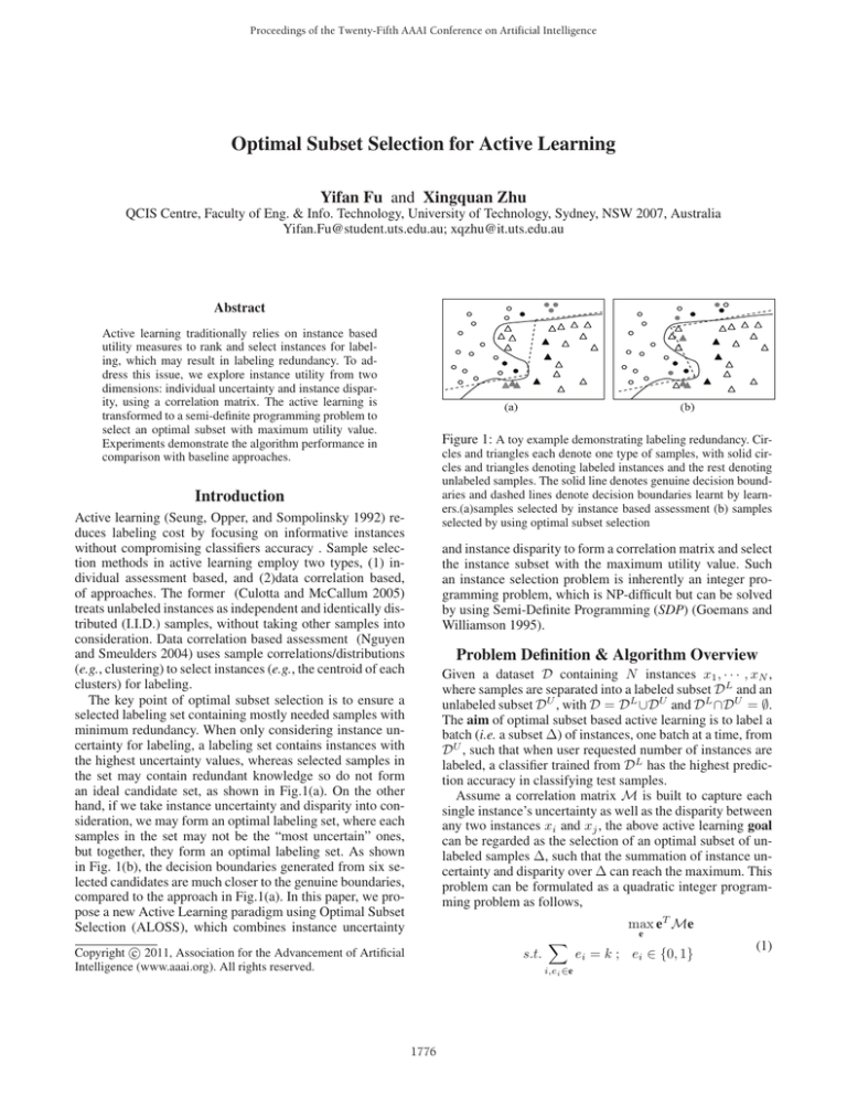
Figure 1: A toy example demonstrating labeling redundancy. Circles and triangles each denote one type of samples, with solid circles and triangles denoting labeled instances and the rest denoting
unlabeled samples. The solid line denotes genuine decision boundaries and dashed lines denote decision boundaries learnt by learners.(a)samples selected by instance based assessment (b) samples
selected by using optimal subset selection
Introduction
Active learning (Seung, Opper, and Sompolinsky 1992) reduces labeling cost by focusing on informative instances
without compromising classifiers accuracy . Sample selection methods in active learning employ two types, (1) individual assessment based, and (2)data correlation based,
of approaches. The former (Culotta and McCallum 2005)
treats unlabeled instances as independent and identically distributed (I.I.D.) samples, without taking other samples into
consideration. Data correlation based assessment (Nguyen
and Smeulders 2004) uses sample correlations/distributions
(e.g., clustering) to select instances (e.g., the centroid of each
clusters) for labeling.
The key point of optimal subset selection is to ensure a
selected labeling set containing mostly needed samples with
minimum redundancy. When only considering instance uncertainty for labeling, a labeling set contains instances with
the highest uncertainty values, whereas selected samples in
the set may contain redundant knowledge so do not form
an ideal candidate set, as shown in Fig.1(a). On the other
hand, if we take instance uncertainty and disparity into consideration, we may form an optimal labeling set, where each
samples in the set may not be the “most uncertain” ones,
but together, they form an optimal labeling set. As shown
in Fig. 1(b), the decision boundaries generated from six selected candidates are much closer to the genuine boundaries,
compared to the approach in Fig.1(a). In this paper, we propose a new Active Learning paradigm using Optimal Subset
Selection (ALOSS), which combines instance uncertainty
and instance disparity to form a correlation matrix and select
the instance subset with the maximum utility value. Such
an instance selection problem is inherently an integer programming problem, which is NP-difficult but can be solved
by using Semi-Definite Programming (SDP) (Goemans and
Williamson 1995).
Problem Definition & Algorithm Overview
Given a dataset D containing N instances x1 , · · · , xN ,
where samples are separated into a labeled subset DL and an
unlabeled subset DU , with D = DL ∪DU and DL ∩DU = ∅.
The aim of optimal subset based active learning is to label a
batch (i.e. a subset Δ) of instances, one batch at a time, from
DU , such that when user requested number of instances are
labeled, a classifier trained from DL has the highest prediction accuracy in classifying test samples.
Assume a correlation matrix M is built to capture each
single instance’s uncertainty as well as the disparity between
any two instances xi and xj , the above active learning goal
can be regarded as the selection of an optimal subset of unlabeled samples Δ, such that the summation of instance uncertainty and disparity over Δ can reach the maximum. This
problem can be formulated as a quadratic integer programming problem as follows,
s.t.
c 2011, Association for the Advancement of Artificial
Copyright Intelligence (www.aaai.org). All rights reserved.
i,ei ∈e
1776
max eT Me
e
ei = k ; ei ∈ {0, 1}
(1)
where e is an n-dimensional column vector and n is the size
of unlabeled set DU . The constraint k defines the size of the
subset for labeling, with ei = 1 denoting that instance xi
is selected for labeling and ei = 0 otherwise. Algorithm 1
describes the general process of our method.
Optimal Subset Selection
Using correlation matrix M, the objective function defined
in Eq.(1) is to select a k instance subset such that the summation of all instances’ uncertainty and their disparities is the
maximum among all alternative subsets with the same size.
This problem is NP-difficult. We use SDP approximation algorithm “Max cut with size k” (MC-k) problem (Goemans
and Williamson 1995) to solve this maximization problem
with polynomical complexity.
Algorithm 1 ALOSS: Active Learning with Optimal Subset
Selection
1: while labeledSample <budget do
2:
construct a classifier ensemble with labeled training set DL ;
3:
Build correlation Matrix M
4:
Apply optimal subset selection to M and select an optimal
subset Δ with k instances;
5:
labeledSample ← labeledSample + k;
6: end while
Experimental Results
In Fig. 2, we compare accuracy between ALOSS and several baseline approaches on ”auto” dataset, where “Entropy”
denotes entropy-based uncertainty sampling (which has the
same batch size Δ as ALOSS) and “SIB” represents Single Instance Batch active learning (which repeats for each
single instance). From Fig. 2, it is clear that Entropy is the
least effective algorithm because it does not take labeling redundancy into consideration. SIB can reduce labeling redundancy to some extent (by labeling instance one at a time), but
it still cannot guarantee an optimal labeling set. By combing
instance uncertainty and disparity to select optimal subsets,
ALOSS outperforms all baseline approaches.
Correlation Matrix Construction
To build a correlation matrix M ∈ Rn×n , where n denotes
the number of instances in the unlabeled set DU , we separate
elements in M into two parts. More specifically, assume Ui,i
defines the uncertainty of instance xi and Ii,j , i = j defines
the disparity between instances xi and xj , the correlation
matrix M is constructed using Eq.(2)
if i = j
Ui,j ,
(2)
Mi,j =
if i = j
Ii,j ,
Instance Uncertainty
To calculate uncertainty for each single instance xi in DU ,
we build a classifier ensemble E with π heterogeneous
members, 1 , · · · , π trained from labeled sample set DL .
Denoting H ∈ Rπ×π a normalized classifier weighting matrix where each element Hi,j denotes the agreement between
classifiers i and j in classifying all instances in DU . After that, we apply each classifier j , j = 1, · · · , π, to xi ,
and build a vector ui with each element ui,j , j = 1, · · · , π,
recording uncertainty of classifier j on instance xi . As a
result, we build an n by π matrix u ∈ Rn×π , and calculate
weighted instance uncertainty as follows.
U = u × H × uT
Figure 2: Algorithms accuracy comparison between ALOSS and
baseline methods w.r.t. different percentages of labeled data
Conclusion
We proposed a new active learning paradigm using optimal
subset selection (ALOSS), which considers uncertainty and
disparity of an instances subset to reduce labeling redundancy and achieve good performance.
(3)
Instance Disparity
We employ two types of distance measures, prediction distance and feature distance, to calculate disparity between
each pair of instances xi and xj .
Prediction Distance (P) captures prediction dissimilarity of
a set of classifiers on two instances. For a pair of instance xi
and xj , their prediction difference is accumulated prediction
distance over all class labels and all classifiers.
Feature Distance (F) captures the disparity of a pair of instances by using their Euclidean distance.
Instance Disparity (I): Because prediction distance (P)
and feature distance (F) each denotes the difference between instances xi vs. xj from different perspectives, the
final disparity between xi and xj is the product of the two
distances as follows.
Ii,j = Pi,j × Fi,j
Acknowledgement
This research is supported by Australian Research Council
Future Fellowship under Grant No. FT100100971.
References
Culotta, A., and McCallum, A. 2005. Reducing labeling effort for
stuctured prediction tasks. In Proc. of AAAI, 746–751.
Goemans, M., and Williamson, D. 1995. Improved approximation algorithms for maximum cut and satisfiability problems using
semidefinite prgramming. J. of ACM 42.
Nguyen, H., and Smeulders, A. 2004. Active learning using preclustering. In Proc. of ICML, 623–630.
Seung, H.; Opper, M.; and Sompolinsky, H. 1992. Query by committee. In Proc. of COLT, 287–294.
(4)
1777