Proceedings of the Twenty-Fourth AAAI Conference on Artificial Intelligence (AAAI-10)
Optimal Rectangle Packing on Non-Square Benchmarks
Eric Huang and Richard E. Korf
Computer Science Department
University of California, Los Angeles
Los Angeles, CA 90095
ehuang@cs.ucla.edu, korf@cs.ucla.edu
Abstract
The rectangle packing problem consists of finding an
enclosing rectangle of smallest area that can contain a
given set of rectangles without overlap. We propose
two new benchmarks, one where the orientation of the
rectangles is fixed and one where it is free, that include
rectangles of various aspect ratios. The new benchmarks avoid certain properties of easy instances, which
we identify as instances where rectangles have dimensions in common or where a few rectangles occupy most
of the area. Our benchmarks are much more difficult
for the previous state-of-the-art solver, requiring orders
of magnitude more time, compared to similar-sized instances from a popular benchmark consisting only of
squares. On the new benchmarks, we improve upon the
previous strategy used to handle dominance conditions,
we define a variable order over non-square rectangles
that generalizes previous strategies, and we present a
way to adjust the sizes of intervals of values for each
rectangle’s x-coordinates. Using these techniques together, we can solve the new oriented benchmark about
500 times faster, and the new unoriented benchmark
about 40 times faster than the previous state-of-the-art.
Introduction
Given a set of rectangles, our problem is to find all enclosing
rectangles of minimum area that will contain them without
overlap. We refer to an enclosing rectangle as a bounding
box. The optimization problem is NP-hard, while the problem of deciding whether a set of rectangles can be packed
in a given bounding box is NP-complete, via a reduction
from bin-packing (Korf 2003). We introduce the oriented
constant-perimeter rectangle packing benchmark, which is
a simple set of increasingly difficult instances for this problem, where the task is to find all bounding boxes of minimum area that contain a set of rectangles of sizes 1xN ,
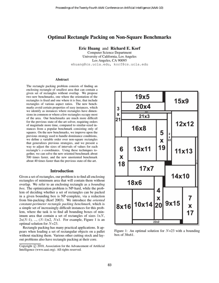
2x(N -1), ..., (N -1)x2, N x1. For example, Figure 1 is an
optimal solution for N =23.
Rectangle packing has many practical applications. It appears when loading a set of rectangular objects on a pallet
without stacking them. Various other cutting stock and layout problems also have rectangle packing at their core.
Figure 1: An optimal solution for N =23 with a bounding
box of 38x61.
c 2010, Association for the Advancement of Artificial
Copyright Intelligence (www.aaai.org). All rights reserved.
83
(a) A dominated position for
the 4x4 square.
(b) An undominated position
for the 4x4 square.
Figure 3: Assigning a 4x2 to [0,2].
Figure 2: Example of dominance conditions.
In contrast to Korf’s (2003) solver, Simonis and
O’Sullivan’s (2008) solver determined the x-coordinates of
the rectangles prior to any of the y-coordinates, as suggested by Clautiaux et al. (2007). Their Prolog program used
the cumulative constraint (Aggoun and Beldiceanu 1993),
which requires that the sum of the heights of all rectangles
overlapping any given x-coordinate never exceeds the height
of the bounding box. Since we use some of these ideas, we
review them here.
Simonis and O’Sullivan (2008) divided the domain of the
x-coordinates for each rectangle into a set of intervals, the
size of which was tuned experimentally. These x-intervals
are explored in turn, and constrain the x-coordinates that
may be assigned to the corresponding rectangle. Committing to an interval also induces a smaller rectangle representing the common intersecting area of placing the rectangle in any location in the interval, similar to the ideas of
Beldiceanu et al. (2008). Larger intervals result in weaker
constraint propagation (less pruning) but a smaller branching factor, while smaller intervals result in stronger constraint propagation but a larger branching factor.
For example, in Figure 3 a 4x2 rectangle assigned an
x-interval of [0,2] consumes 2 units of area at each xcoordinate in [2,3], represented by the doubly-hatched area,
regardless of where it is placed in the interval. This compulsory part (Lahrichi 1982) is a constraint common to all positions x ∈ [0, 2] of the original 4x2 rectangle. If there were
no feasible set of interval assignments, then finding individual x-values would be unnecessary. However, if we do find
a set of interval assignments, then we will have to search for
a set of single x-coordinate values. Simonis and O’Sullivan
(2008) assigned (in order) x-intervals, single x-coordinates,
y-intervals, and finally single y-coordinates.
Our previous solver (Huang and Korf 2009) outperformed
that of Simonis and O’Sullivan by solving the y-coordinates
differently. For every x-coordinate solution, we would solve
a perfect packing instance to find the y-coordinates. A perfect packing problem is a rectangle packing problem with
the property that the solution has no empty space, and such
an instance is created by adding to the original set of rectangles a number of 1x1 rectangles equal to the area of empty
space in the original instance.
Rectangle packing may also model some scheduling problems where tasks consume resources that must be allocated
in contiguous chunks. For example, consider the task of
scheduling when ships should berth at various locations
along one long wharf. The time a ship remains docked may
be represented as the width of a rectangle while the ship’s
length may be represented as its height. A rectangle packing solution then tells us where and when ships should be
berthed. One can similarly model other problems where resources should be allocated contiguously to tasks that require them, such as memory or radio frequency spectrum.
Previous Work
Korf (2003) divided the rectangle packing problem into two
subproblems: the containment problem and the minimal
bounding box problem. The former tries to pack the given
rectangles in a given bounding box, while the latter finds a
bounding box of least area that can contain a given set of
rectangles. The algorithm that solves the minimal bounding
box problem calls the algorithm that solves the containment
problem as a subroutine.
Containment Problem
Korf’s (2003) absolute placement approach modeled rectangles as variables and positions in the bounding box as values.
He introduced a set of dominance conditions to prune positions where large rectangles are too close to the sides of the
bounding box. For example, imagine that we must pack the
squares 4x4, 3x3, 2x2, and 1x1. In Figure 2a, the 4x4 placed
at x=2 leaves a 2x4 gap against the left side of the bounding
box in which the 3x3 cannot fit. Only the 2x2 and 1x1 can fit
within the gap, and in fact they both can be placed entirely
within the gap simultaneously.
Now notice that in any solution with the 4x4, 2x2, and
1x1 arranged as in Figure 2a, we can always rearrange them
as in Figure 2b without disturbing any other squares. Thus,
as long as we have tried placing the 4x4 at x=0, we would
not have to try x=2, because if there were a solution at x=2
then we would have found it earlier when trying x=0. In
general, a position for a rectangle is dominated if it leaves a
gap in which all rectangles that can individually fit can also
be packed together in the gap without protruding from it.
This guarantees they can be swapped as in Figure 2 (Korf
2003).
Minimal Bounding Box Problem
A simple way to solve the minimal bounding box problem
is as follows. The minimum height and width of any feasible bounding box is determined by the maximum height
84
and maximum width, respectively, of the given rectangles.
The maximum width is found by computing a greedy solution with the minimum height, and the maximum height is
found by a greedy solution with the minimum width. Such a
greedy solution is computed by placing the rectangles in the
first available position when scanning from left to right, and
for each column scanning from bottom to top.
We then generate a bounding box for each pair of width
and height in these ranges, rejecting any box whose area
is less than the sum of the rectangle areas. For some box
heights, some rectangles cannot be stacked on top of each
other, so they must be placed side-by-side, giving us a minimum width. We reject any box whose width is less than
the minimum width for its height, and reject any box whose
height is less than the minimum height for its width. The
remaining boxes are sorted in non-decreasing order of area,
and tested one by one, until a feasible solution is found. If
all optimal solutions are desired, we test all bounding boxes
whose area equals that of the optimal solution.
(a) Solution in a 21x35
bounding box for the unoriented instance 1x2, 2x3, ...,
11x12, 12x13.
Rectangle Packing Benchmarks
(b) Solution in a 14x26
bounding box for the unoriented instance 1x12, 2x11,
..., 11x2, 12x1.
Figure 4: Examples of solutions for instances where rectangles may have the same dimensions.
The previous state-of-the-art used the consecutive-square
packing benchmark (Korf 2003), a simple set of increasingly
difficult instances for this problem, where the task is to find
all bounding boxes of minimum area that contain a set of
squares of sizes 1x1, 2x2, ..., up to N xN . Another benchmark used in the literature is the unoriented rectangle packing benchmark (Korf, Moffitt, and Pollack 2009), in which
an instance is a set of rectangles of sizes 1x2, 2x3, ..., up to
N x(N +1), and rectangles may be rotated by 90-degrees.
Properties of Easy Benchmarks
Two Harder Benchmarks
There are several explanations for why the previous benchmarks are easier than our new ones. For the reasons we will
subsequently explain, we have constructed our new benchmarks to describe instances consisting of rectangles with
unique dimensions, without duplicates, and where most of
the area is not captured by only a few rectangles.
We propose two new benchmarks that demonstrate limitations of using only the consecutive-square and unoriented
rectangle packing benchmarks to compare previous solvers.
The first is the oriented constant-perimeter rectangle packing benchmark, where instances are described as a set of
rectangles of sizes 1xN , 2x(N -1), ..., (N -1)x2, N x1, and
rectangles may not be rotated. Given a parameter N , all
rectangles are unique and have a perimeter of 2N +2. The
second is the unoriented constant-perimeter rectangle packing benchmark, where instances are described as a set of
rectangles 1x(2N -1), 2x(2N -2), ..., (N -1)x(N +1), N xN ,
and rectangles may be rotated by 90-degrees. All rectangles
here are unique and have a perimeter of 4N .
Both of these new benchmarks are much more difficult
than either the consecutive-square packing benchmark or the
unoriented rectangle benchmark (Korf, Moffitt, and Pollack
2009). We tested our former state-of-the-art solver (Huang
and Korf 2009) on both old and new benchmarks. Solving
N =21 of our oriented constant-perimeter benchmark took
almost four days, while instances with the same number of
rectangles from the consecutive-square and unoriented rectangle packing benchmarks took only one second and eight
seconds, respectively. Our unoriented constant-perimeter
benchmark was even more difficult in that the largest size
we could run using our previous solver was N =16, taking
over 40 hours.
Rectangles With Equal Dimensions In the old unoriented rectangle benchmark, all instances have rectangles that
share some dimension with another rectangle. For example,
Figure 4a is an optimal solution of N =12. In all optimal solutions up to the largest we can run, rectangles equal in some
dimension tend to line up next to each other, forming larger
rectangles and leaving little empty space. In Figure 4a, the
8x9 and 8x7 line up, as do the 6x5 with the 4x5, and the 3x4
with the 3x2. Note also that the 6x5, 4x5, 3x4, 3x2 and 7x6
together form a larger 10x11 rectangle with no empty space.
In fact, the optimal solutions in this benchmark all have
much less empty space than similar-sized instances from
the consecutive-square packing benchmark, where all rectangles have unique dimensions. Note that this is not an intrinsic property of a benchmark that is unoriented, but this
happens to be a property that exists in the unoriented rectangle packing benchmark proposed by Korf et al. (2009).
We have also considered a benchmark whose instances
contain duplicate rectangles. For example, take any instance
from our oriented constant-perimeter benchmark, and simply allow the rectangles to be rotated 90-degrees. Figure 4b
is a solution to one such instance. Here, there are always
two identical rectangles in every instance, except for the occasional single square. Note that having duplicate rectangles
is a special case of having rectangles with equal dimensions,
which is why we see the rectangles lining up to form larger
85
In our constant-perimeter benchmarks, the 1xN rectangle
can always partially fit in gaps left by other rectangles, but it
must always protrude out of those gaps, thereby eliminating
the dominance conditions we previously described. Without any dominated positions to account for, our old solver
ends up committing to single x-coordinate values in a situation where it is more desirable to include those positions in a
larger interval assignment. In addition to dynamically inferring dominance rules, our new solver detects when there are
no dominated positions and adjusts the interval assignments
to avoid this behavior.
rectangles. Furthermore, the presence of duplicates allows
additional symmetry-breaking techniques such as forcing
the x-coordinate value of one rectangle to be greater than
or equal to that of its duplicate.
The optimal solution is found rapidly on instances with
these properties. Since our solver tests bounding boxes in
non-decreasing order of area, and since the optimal solutions
of these easy instances have very little empty space, we test
and find the optimal bounding boxes very early.
Rectangles With Little Area and Small Dimensions In
both the consecutive-square and the unoriented rectangle
packing benchmarks, a few large rectangles capture much
of an instance’s total area. Thus, the solver does not search
too deeply before using up the allowable empty space. With
little empty space, backtracking is very likely since we cannot find a place for the next rectangle. Therefore, small rectangles in these benchmarks may not matter for much of the
search effort.
Previous benchmarks such as the consecutive-square
packing benchmark described rectangles of small area with
both small widths and small heights, and those of large area
with large widths and heights, making it obvious to place
large rectangles first because they are the most constrained
variables as well as have the most constraining values.
By contrast, in our new benchmarks there is a trade-off
between rectangles with large dimensions and those with
large area. The widest rectangle in our oriented constantperimeter benchmark has the smallest branching factor as
we search for x-coordinates. However, it also has the least
area, so during search it won’t constrain the cumulative constraint much. This raises the non-trivial question of how to
define a good variable order over non-square rectangles.
Ordering Variables By Branching Factor
There is a natural variable order that arises from both the
consecutive-square and unoriented rectangle packing benchmarks when using the strategy of picking the most constrained variable next. No matter which property we use to
determine the most constrained variable – height, width, or
area – all properties agree on placing rectangles in decreasing order of size. In our new benchmarks, however, it is not
obvious what variable order to use.
We propose a variable order over rectangles of various
aspect ratios by picking the most constrained variable first,
to favor a smaller branching factor closer to the root of the
search tree. For the oriented constant-perimeter benchmark,
recall that we assign intervals to the x-coordinates before
the y-coordinates, and like Simonis and Sullivan (2008) we
use a constant factor times the rectangle width to define the
interval size. This means the branching factor for the xinterval variables for a given rectangle is
Bw − rw
Bw 1
1
b=
=
− ,
Crw
C rw
C
New Solution Strategies
(1)
where Bw is the bounding box width, rw is the rectangle
width, and C is a constant chosen experimentally. The numerator Bw − rw is the number of x-coordinate values that
the rectangle may assume while still fitting in the bounding box, and the denominator Crw is the size of the interval
we will be assigning to the given rectangle. For example, if
C=0.75 then we would assign intervals of size three to a 4x2
rectangle.
We may drop the translational constant −1/C as well
as the positive scalar Bw /C, because doing so would not
change the relative ordering of the rectangles prescribed by
the function. This leaves us with 1/rw , which means that
for the oriented benchmark we should place the rectangles
in order of decreasing width.
For the unoriented constant-perimeter benchmark, our
solver first tries all values for a particular x-interval, and
then rotates the rectangle 90-degrees before trying another
set of x-interval values. In this case the branching factor is
We improve upon our previous state-of-the-art solver with
the following techniques, which help in solving the new
benchmarks.
Instances Without Dominance Conditions
On the consecutive-square packing benchmark, our previous
solver used intervals for the x-coordinates only on undominated positions. For example, a 20x20 square in a bounding
box of width 42 has an x-coordinate domain of x={0, [6,16],
22} because we specifically exclude the dominated positions
x={[1,5], [17,21]} as we try different interval assignments.
Here, the first x-interval assignment that we branch on will
just be the single-valued interval x=[0,0], since it is useless
to include any values from [1,5]. The same thing also occurs
at the right side of the bounding box. Therefore, the solver
only makes non-trivial interval assignments for the domain
x={[6,16]}, representing the interior of the bounding box.
While this technique improved the performance for consecutive-square packing by a factor of five compared to
leaving it out, it actually slowed the performance on our
new benchmarks by the same factor. This occurs because
the dominant positions, such as placing the rectangle flush
against the left or right sides of the bounding box, are always explored by committing to single x-coordinate values.
Bw − rw
Bw − rh
Bw 1
1
2
b=
+
=
+
− . (2)
Crw
Crh
C rw
rh
C
As mentioned before, we can drop the positive scalar and
translational constant, giving us
86
Size
N
Optimal
Solution
Empty
Space
Boxes
Tested
13
14
15
16
17
18
19
20
21
22
23
16×29
19×30, 15×38
24×29
23×36
24×41
24×48
32×42, 24×56
37×42
35×51
34×60
38×61
1.94%
1.75%
2.30%
1.45%
1.52%
1.04%
1.04%
0.90%
0.78%
0.78%
0.78%
7
7
10
9
8
12
12
11
9
15
16
HK09
Time
NoDom
Time
BrFactor
Time
C=0.55
Time
HK10
Time
:01
:02
:16
:57
5:56
1:06:32
6:35:48
1:18:51:34
3:21:31:46
:00
:01
:05
:16
1:21
14:47
1:26:16
7:36:09
13:33:16
:00
:00
:01
:02
:27
6:15
31:23
1:51:10
4:22:49
:00
:00
:00
:00
:03
:32
3:34
13:06
20:49
14:22:03
:00
:00
:00
:00
:02
:22
2:15
7:51
11:20
9:12:37
3:22:50:38
Table 1: Minimum-area bounding boxes containing all oriented rectangles 1xN , 2x(N -1), ..., (N -1)x2, N x1.
fraction of empty space in the optimal solution. The fourth
gives the number of bounding boxes that were tested to find
all optimal solutions. The remaining columns represent the
CPU times for each solver in the format of days, hours, minutes, and seconds. We wrote our solver in C++ and collected
our data on a 2.93GHz Intel Core 2 Duo E7500 using only
one core, one process, and one thread.
From left to right, each successive solver improves on
the previous one by including an additional technique.
The column called HK09 is data collected using our old
code (Huang and Korf 2009). Since the previous literature
did not define a variable order over non-squares, we used the
order of decreasing area by default.
NoDom improves upon HK09 in that it detects when no
dominated positions exist and therefore includes the dominant positions with the interval assignments. BrFactor improves upon NoDom in that it orders the oriented constantperimeter benchmark by decreasing width and the unoriented constant-perimeter benchmark by decreasing area.
C=0.55 improves upon BrFactor in that we use an interval
size of 0.55 instead of C=0.35 as recommended in previous literature. Finally, HK10 improves upon C=0.55 in that
it uses knowledge of the branching factor to rebalance the
sizes of the interval assignments for the x-coordinates.
Notice that NoDom, BrFactor, and C=0.55 introduce
techniques that reduce the branching factor, and so they have
a greater effect on performance than HK10, whose new technique seeks to make the intervals assigned equally constraining. Our experiments reveal that these techniques interact
with one another, and we note that without including dominated positions in the intervals, the performance gained from
the other techniques appear muted. This interaction is also
why we tune the global interval parameter C only after including the other techniques that affect the branching factor.
Ordering by branching factor made a significant difference for our oriented constant-perimeter benchmark but not
for our unoriented benchmark. For the unoriented benchmark, we omit a column for BrFactor in Table 2 because ordering by branching factor prescribes ordering by decreasing
area, which is what we gave the solver by default.
Note that the unoriented constant-perimeter benchmark
1
1
rw + rh
+
=
.
(3)
rw
rh
rw rh
Because all rectangles in a given instance have the same
perimeter by definition, the numerator of the result in Equation 3 is constant. Therefore for our unoriented benchmark,
we would place the rectangles in order of decreasing area.
Larger and Balanced Interval Sizes
Our old solver used an interval size that is 0.35 times the
width of a given rectangle. We have found that larger interval sizes improve the performance of our solver on the new
benchmarks, and use a value of C=0.55 instead.
As we assign larger intervals to the short and wide rectangles, the x-interval variables for these rectangles tend to
have branching factors of three or less. Here, we should balance the sizes of these intervals so that the values assigned
are equally constraining on their subtrees. For example, consider C=0.55, a rectangle of width 20, and its set of possible x-coordinate values [0,23]. Our previous state-of-theart would try intervals containing eleven values each, first
branching on x=[0,10] and x=[11,21], and then exploring
the remaining interval x=[22,23]. This results in small compulsory parts in the first two branches, but a very large one
in the third.
Since we must explore three branches anyway, we can
balance the sizes of these interval assignments by exploring
x=[0,7], x=[8,15], and x=[16,23]. Our solver first computes
the branching factor induced by the global interval parameter C=0.55 for each rectangle, and then it balances the number of values in each interval assignment.
Experimental Results
Table 1 compares the performance of our previous stateof-the-art on the oriented constant-perimeter benchmark
against different versions of our solver. Table 2 compares
the same solvers using our unoriented constant-perimeter
benchmark. The first column is the number of rectangles.
The second gives the optimal bounding boxes (some instances have multiple optimal solutions). The third gives the
87
Size
N
Optimal
Solution
Empty
Space
Boxes
Tested
11
12
13
14
15
16
17
18
29×33
21×59
38×41
38×51, 17×114
44×54
45×64, 30×961
39×88, 52×66
55×74
1.15%
1.37%
0.71%
0.67%
0.67%
0.83%
0.44%
0.57%
12
17
13
17
21
35
27
35
HK09
Time
NoDom
Time
C=0.55
Time
HK10
Time
:01
:20
1:45
28:48
1:43:01
1:16:46:44
:00
:04
:21
4:53
11:36
4:13:34
1:12:40:14
:00
:01
:06
1:19
3:33
1:16:02
9:44:14
:00
:01
:06
1:15
2:34
1:01:54
7:53:50
2:02:10:38
Table 2: Minimum-area bounding boxes containing all unoriented rectangles 1x(2N -1), 2x(2N -2), ..., (N -1)x(N +1), N xN .
packing benchmark with the same number of rectangles.
We therefore advocate the use of these benchmarks for research in optimal rectangle packing as they appear to be
significantly more difficult than the benchmarks used in the
previous literature. Finally, using all of our techniques together we are able to solve N =21 of the oriented constantperimeter benchmark about 500 times faster and N =16
of the unoriented constant-perimeter benchmark about 40
times faster than the previous state-of-the-art.
requires our solver to try approximately twice as many
bounding boxes for a given parameter N than that required
for our oriented benchmark. This is due to having 2N -1
as the largest dimension in the unoriented benchmark while
having N as the largest dimension in the oriented benchmark. Since we generate and test all bounding boxes with
widths and heights within computed ranges, instances described with large integers result in more bounding boxes
that must be tested. Thus, an instance with N rectangles in
this benchmark is incomparable to an instance of N squares
from the consecutive-square packing benchmark when evaluating benchmark difficulty. Still, the difference in the number of bounding boxes tested cannot fully account for the orders of magnitude of additional time that the previous stateof-the-art solver requires.
Finally, we also tested our new solver on the consecutivesquare packing benchmark to see the effects of any extra
overhead added by our improvements. Our new solver resulted in only a five percent speedup compared to our old
solver, likely due to minor improvements in data structures,
and balancing interval sizes.
In summary, using all of our techniques together, we can
solve N =21 of the oriented constant-perimeter benchmark
about 500 times faster and N =16 of the unoriented constantperimeter benchmark about 40 times faster than the previous
state-of-the-art.
Acknowledgments
This research was supported in part by NSF grant No. IIS0713178.
References
Aggoun, A., and Beldiceanu, N. 1993. Extending chip in
order to solve complex scheduling and placement problems.
Mathematical and Computer Modelling 17(7):57 – 73.
Beldiceanu, N.; Carlsson, M.; and Poder, E. 2008. New
filtering for the cumulative constraint in the context of nonoverlapping rectangles. In Perron, L., and Trick, M. A., eds.,
CPAIOR, volume 5015 of Lecture Notes in Computer Science, 21–35. Springer.
Clautiaux, F.; Carlier, J.; and Moukrim, A. 2007. A
new exact method for the two-dimensional orthogonal packing problem. European Journal of Operational Research
183(3):1196 – 1211.
Huang, E., and Korf, R. E. 2009. New improvements in
optimal rectangle packing. In Boutilier, C., ed., IJCAI, 511–
516.
Korf, R.; Moffitt, M.; and Pollack, M. 2009. Optimal rectangle packing. To appear in Annals of Operations Research.
Korf, R. E. 2003. Optimal rectangle packing: Initial results.
In Giunchiglia, E.; Muscettola, N.; and Nau, D. S., eds.,
ICAPS, 287–295. AAAI.
Lahrichi, A. 1982. Scheduling: the notions of hump, compulsory parts and their use in cumulative problems. C.R.
Acad. Sci., Paris 294:209–211.
Simonis, H., and O’Sullivan, B. 2008. Search strategies for
rectangle packing. In Stuckey, P. J., ed., CP, volume 5202
of Lecture Notes in Computer Science, 52–66. Springer.
Conclusion
We have introduced two new benchmarks, one oriented and
one unoriented, that include rectangles of various aspect ratios. These new benchmarks avoid various properties of easy
instances, which we have identified. We have also proposed
several search strategies to improve performance on our new
benchmarks. We improved upon the previous strategy used
to handle dominance conditions, proposed a variable ordering heuristic based on increasing branching factor that generalizes previous strategies, tuned a global interval parameter, and introduced a method to balance the sizes of the
intervals assigned to the x-coordinate variables.
Our experiments reveal that the previous state-of-the-art
takes orders of magnitude more time to solve our new benchmarks compared to instances from the consecutive-square
1
40×72 and 48×60 are also optimal solutions.
88