Proceedings of the Sixth International Symposium on Combinatorial Search
Frequency Data Compression for Public
Transportation Network Algorithms (Extended Abstract)
Hannah Bast and Sabine Storandt
Albert-Ludwigs-Universität Freiburg
Institut für Informatik
79110 Freiburg, Germany
bast,storandt@informatik.uni-freiburg.de
Abstract
S314
Timetable information in public transportation networks exhibit a large degree of redundancy; e.g. consider a bus going from station A to station B at 6:00, 6:15, 6:30, 6:45,
7:00, 7:15, 7:30, . . . , 20:00, the very same data can be provided by a frequency-based representation as ’6:00-20:00,
every 15 minutes’ in considerably less space. Nevertheless
a common graph model for routing in public transportation
networks is the time-expanded representation where for each
arrival/departure event a single node is created. We will introduce a frequency-based graph model which allows for a
significantly more compact representation of the network, resulting also in a speed-up for station-to-station queries. Moreover we will describe a new variant of Dijkstra’s algorithm,
where also the labels are frequency-based. This approach allows for accelerating profile queries in public transportation
networks.
R6
A
S205
0
X
0
D
TB
S99
([6:00,22:00],5min,14min)
R12
R12
0
0
A
0
TB
X
0
0
0
6min
0
TB
0
8min
0
([6:00,22:00],5min, 3min)
R12
0
0
0 TB
D
TB
0
A
0
([8:00,23:00],15min, 12min)
R87
X
0
D
TB
0
R87
([5:00,8:15],25min,16min)
Introduction
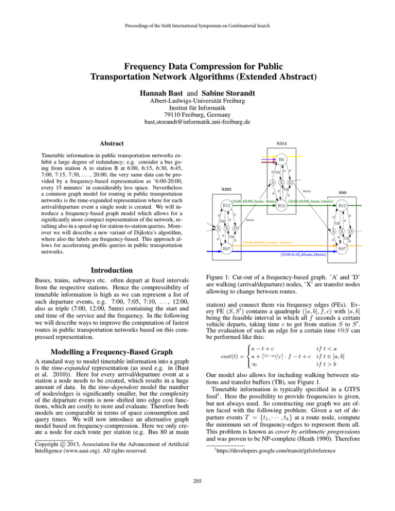
Figure 1: Cut-out of a frequency-based graph. ’A’ and ’D’
are walking (arrival/departure) nodes, ’X’ are transfer nodes
allowing to change between routes.
Buses, trains, subways etc. often depart at fixed intervals
from the respective stations. Hence the compressibility of
timetable information is high as we can represent a list of
such departure events, e.g. 7:00, 7:05, 7:10, . . . , 12:00,
also as triple (7:00, 12:00, 5min) containing the start and
end time of the service and the frequency. In the following
we will describe ways to improve the computation of fastest
routes in public transportation networks based on this compressed representation.
station) and connect them via frequency edges (FEs). Every FE (S, S 0 ) contains a quadruple ([a, b], f, c) with [a, b]
being the feasible interval in which all f seconds a certain
vehicle departs, taking time c to get from station S to S 0 .
The evaluation of such an edge for a certain time t@S can
be performed like this:


a − t + c
cost(t) = a + d(t−a)/f e · f − t + c

∞
Modelling a Frequency-Based Graph
A standard way to model timetable information into a graph
is the time-expanded representation (as used e.g. in (Bast
et al. 2010)). Here for every arrival/departure event at a
station a node needs to be created, which results in a huge
amount of data. In the time-dependent model the number
of nodes/edges is significantly smaller, but the complexity
of the departure events is now shifted into edge cost functions, which are costly to store and evaluate. Therefore both
models are comparable in terms of space consumption and
query times. We will now introduce an alternative graph
model based on frequency-compression. Here we only create a node for each route per station (e.g. Bus 80 at main
if t < a
if t ∈ [a, b]
if t > b
Our model also allows for including walking between stations and transfer buffers (TB), see Figure 1.
Timetable information is typically specified in a GTFS
feed1 . Here the possibility to provide frequencies is given,
but not always used. So constructing our graph we are often faced with the following problem: Given a set of departure events T = {t1 , · · · , tk } at a route node, compute
the minimum set of frequency-edges to represent them all.
This problem is known as cover by arithmetic progressions
and was proven to be NP-complete (Heath 1990). Therefore
c 2013, Association for the Advancement of Artificial
Copyright Intelligence (www.aaai.org). All rights reserved.
1
205
https://developers.google.com/transit/gtfs/reference
#stations
#departure events
#freqeuncy-edges
compression factor
Manhattan
1831
278920
87505
3.2
Toronto
10891
1599746
315300
5.1
3. Compute for the first steps = lcm/lf relevant departure
times {start, start + lf , · · · , start + (steps − 1) · lf }
(restricted to values ≤ lb ) the explicit edge costs cost and
arrival times arr at v. Store the respective values in a
vector A.
4. Parse through A and remove arrival times, which occur
more than once (of course keeping the one with the lowest cost); but be careful, that the last connection is not
among the pruned ones (if so, add this single connection
manually).
5. For every remaining item in A, create a new label l0 at
node v, with la0 = arr, lb0 = la0 + b(min(lb , eb ) − la0 +
cost)/lcmc · lcm, lf0 = lcm and lc0 = lc + cost.
Table 1: Heuristic frequency-graph construction.
we propose a heuristic strategy: At first, we sort T increasingly. Then we consider the first element t1 and compute the
longest possible arithmetic progression (AP) starting with
t1 . We add this AP to our solution and mark all other elements in T covered by it. Now we repeat the approach
with the next unmarked element. We do not exclude already
marked ones from the set, but we give preference to the AP
which covers the most unmarked elements. Example:
3
1
5
2
7
3
[6:45,10:45], f=15min, c=2h30min
[8:05,20:05], f=20min, c=8min
10 15 17 19 20 23 24 30 31 40 50 60
4
5
The resulting reduction of FEs can be found for two realworld examples in Table 1. Because a FE can be evaluated
in constant time, the compression factor translates into the
speed-up for station-to-station queries.
[8:13,10:13], f=60min, c=2h43min
[8:33,10:33], f=60min, c=2h48min
[8:53,10:53], f=60min, c=2h38min
lcm(15, 20) = 60
start = 8 : 00
steps = 60/15 = 4
dep
8:00
8:15
8:30
8:45
→
→
→
→
arr
8:13,
8:33,
8:53,
8:53,
cost
c=13min
c=18min
c=23min
c= 8min
Profile Queries on Frequency Data
Figure 2: Example of a frequency-edge relaxation.
Profile queries play an important role e.g. in the construction of transfer patterns (Bast et al. 2010), a state-of-the-art
speed-up technique for routing in transit networks. In a profile query, we are given a set of departure times T (e.g. all
departures over the day) at a station S and want to know
for each t ∈ T the optimal connections to all other stations. Naively we could run a complete Dijkstra for every
t ∈ T from the ’A’-node of S, resulting in a runtime of
O(|T |n log(n) + |T |m). In practice this can be improved by
considering the values in T from latest to earliest and storing
along with every node the earliest arrival time assigned so
far. If with an earlier departure time the earliest arrival time
at some node v can not be improved, then v must not be further explored. But even in this scenario, if the basic data exhibits frequency-based departure times, we repeat the same
set of operations again and again (only with a time shift).
Hence we would like a single Dijkstra handling all these departure times at once. For this purpose we assign quadruples
([a, b], f, c) to the nodes instead of single values, with [a, b]
marking the interval of arrival times with frequency f , and
c being the summed costs since the departure from S. The
crucial task is adapting the edge relaxation to this new setting. So given a label l = ([la , lb ], lf , lc ) at node u ∈ V and
an edge e = (u, v) ∈ E with ([ea , eb ], ef , ec ), the goal is
to compute the respective label(s) at node v. We proceed in
five steps (see Figure 2 for an example):
1. Compute lcm = lcm(lf , ef ) to get the lowest common
frequency.
2. Compute the first relevant start time start at u. If la ≥
ea , it yields start = la (if la > eb the edge must no be
considered at all). Otherwise if la < ea then start =
la + b(ea − la )/lf c · lf . If this would result in the start
value exceeding lb we reset it to lb .
So the runtime of an edge relaxation is in O(max(lf , ef )),
and at most lcm/lf new labels are created at v (but obviously never more than the number of departure events at
the source station). For walking edges and edges adjacent
to transfer nodes (which can always be used immediately),
it is not necessary to perform lcm = lcm(lf , ef ) = lf
expanding steps. Instead the relaxation leads to exactly
one new label at v which can be determined directly as
l0 = ([la + ec , lb + ec ], lf , lc + ec ).
Of course not all labels created at the target node must represent (temporary) optimal connections. Therefore the resulting labels have to be pruned properly and joined if possible
to reduce the space consumption.
The respective runtimes of our approach for an implementation in C++ on an Intel i5-3360M CPU with 2.80GHz and
16GB RAM can be found in Table 2.
#stations / #departures
naive
frequency-based
speed-up
Madrid
4653 / 1.20M
26.83
5.98
4.48
Artificial
750 / 0.23M
28.05
0.49
56.39
Table 2: Averaged runtime for 100 profile queries from random source stations in seconds.
References
Bast, H.; Carlsson, E.; Eigenwillig, A.; Geisberger, R.; Harrelson, C.; Raychev, V.; and Viger, F. 2010. Fast routing
in very large public transportation networks using transfer
patterns. In Algorithms–ESA 2010. Springer. 290–301.
Heath, L. S. 1990. Covering a set with arithmetic progressions is NP-complete. Inf. Process. Lett. 34(6):293–298.
206