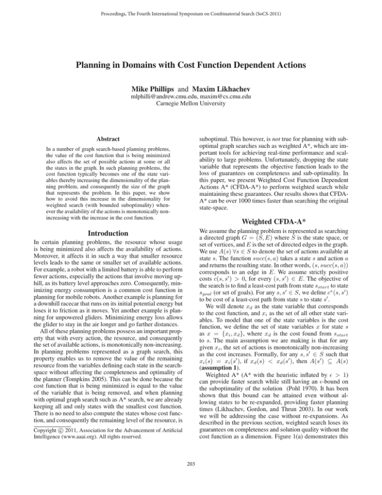
Proceedings, The Fourth International Symposium on Combinatorial Search (SoCS-2011)
Planning in Domains with Cost Function Dependent Actions
Mike Phillips and Maxim Likhachev
mlphilli@andrew.cmu.edu, maxim@cs.cmu.edu
Carnegie Mellon University
suboptimal. This however, is not true for planning with suboptimal graph searches such as weighted A*, which are important tools for achieving real-time performance and scalability to large problems. Unfortunately, dropping the state
variable that represents the objective function leads to the
loss of guarantees on completeness and sub-optimality. In
this paper, we present Weighted Cost Function Dependent
Actions A* (CFDA-A*) to perform weighted search while
maintaining these guarantees. Our results shows that CFDAA* can be over 1000 times faster than searching the original
state-space.
Abstract
In a number of graph search-based planning problems,
the value of the cost function that is being minimized
also affects the set of possible actions at some or all
the states in the graph. In such planning problems, the
cost function typically becomes one of the state variables thereby increasing the dimensionality of the planning problem, and consequently the size of the graph
that represents the problem. In this paper, we show
how to avoid this increase in the dimensionality for
weighted search (with bounded suboptimality) whenever the availability of the actions is monotonically nonincreasing with the increase in the cost function.
Weighted CFDA-A*
We assume the planning problem is represented as searching
a directed graph G = (S, E) where S is the state space, or
set of vertices, and E is the set of directed edges in the graph.
We use A(s) ∀s ∈ S to denote the set of actions available at
state s. The function succ(s, a) takes a state s and action a
and returns the resulting state. In other words, (s, succ(s, a))
corresponds to an edge in E. We assume strictly positive
costs c(s, s ) > 0, for every (s, s ) ∈ E. The objective of
the search is to find a least-cost path from state sstart to state
sgoal (or set of goals). For any s, s ∈ S, we define c∗ (s, s )
to be cost of a least-cost path from state s to state s .
We will denote xd as the state variable that corresponds
to the cost function, and xi as the set of all other state variables. To model that one of the state variables is the cost
function, we define the set of state variables x for state s
as x = {xi , xd }, where xd is the cost found from sstart
to s. The main assumption we are making is that for any
given xi , the set of actions is monotonically non-increasing
as the cost increases. Formally, for any s, s ∈ S such that
xi (s) = xi (s ), if xd (s) < xd (s ), then A(s ) ⊆ A(s)
(assumption 1).
Weighted A* (A* with the heuristic inflated by > 1)
can provide faster search while still having an -bound on
the suboptimality of the solution (Pohl 1970). It has been
shown that this bound can be attained even without allowing states to be re-expanded, providing faster planning
times (Likhachev, Gordon, and Thrun 2003). In our work
we will be addressing the case without re-expansions. As
described in the previous section, weighted search loses its
guarantees on completeness and solution quality without the
cost function as a dimension. Figure 1(a) demonstrates this
Introduction
In certain planning problems, the resource whose usage
is being minimized also affects the availability of actions.
Moreover, it affects it in such a way that smaller resource
levels leads to the same or smaller set of available actions.
For example, a robot with a limited battery is able to perform
fewer actions, especially the actions that involve moving uphill, as its battery level approaches zero. Consequently, minimizing energy consumption is a common cost function in
planning for mobile robots. Another example is planning for
a downhill racecar that runs on its initial potential energy but
loses it to friction as it moves. Yet another example is planning for unpowered gliders. Minimizing energy loss allows
the glider to stay in the air longer and go farther distances.
All of these planning problems possess an important property that with every action, the resource, and consequently
the set of available actions, is monotonically non-increasing.
In planning problems represented as a graph search, this
property enables us to remove the value of the remaining
resource from the variables defining each state in the searchspace without affecting the completeness and optimality of
the planner (Tompkins 2005). This can be done because the
cost function that is being minimized is equal to the value
of the variable that is being removed, and when planning
with optimal graph search such as A* search, we are already
keeping all and only states with the smallest cost function.
There is no need to also compute the states whose cost function, and consequently the remaining level of the resource, is
c 2011, Association for the Advancement of Artificial
Copyright Intelligence (www.aaai.org). All rights reserved.
203
7
(a)
Edge
only
dge on
exists
for g(s1)<α
5
4
Weighted CFDA−A*
3
Weighted A*
1
0
−1
−2
Weighted CFDA−A*
−3
2
Long path
h
_ −4
<
1
1
2
log10(time (s))
log10(expands)
Some
graph
3
Weighted A*
6
2
3
4
5
1
epsilon
(a)
Some
graph
(b)
2
3
4
5
epsilon
(b)
Figure 3: Planning for a limited battery comparing the full state
space and our reduced state space over various . (a) Average expansions (on the log10 scale). (b) Average seconds (on the log10
scale). When the plot drops below the breaks, the planning time
was less than or equal to 0.0001 (≤ −4 on the log10 scale) seconds
and was too small to measure.
Edge
dge on
only
exists
for g(s1)<α
Figure 1: (a) Running normal weighted A* on this graph may return no solution if s1 is expanded sub-optimally (due to inflated
heuristic) such that its g-value exceeds α. On expansion, the state’s
sub-optimal g-value prevents the action from s1 to s2 from being
generated. (b) For a similar reason, the sub-optimality bound can
be violated on this graph if the cost of the long path is greater than
times the minimum cost of the lower path.
of this domain is x, y, energy consumed. There is an energy consumption limit (when the battery is exhausted). The
heuristic used was Euclidean distance. We compare full state
space weighted A* against our weighted CFDA-A*. The
graph shown in Figure 3(a) shows CFDA-A* with up to
1000 times less expansions for smaller . After = 4.0, the
two are similar, because the cost function becomes so dominated by the heuristic (particularly because the max cell cost
is only 6) that both methods end up expanding a straight line
from the start to the goal. Figure 3(b) shows that the actual
planning times have roughly the same speed up as the expansions.
1 g(ŝstart ) = 0; O(ŝstart ) = true; OPEN = ∅; CLOSED = ∅;
2 insert ŝstart into OPEN with f (ŝstart ) = ∗ h(ŝstart );
3 while(ŝgoal is not expanded)
4
remove ŝ with the smallest f -value from OPEN and insert ŝ in CLOSED;
5
s = {xi (ŝ), g(ŝ)};
6
If O(ŝ) = true then Opt = {true, f alse}, else Opt = {f alse}
7
for each a in A(s)
8
s = succ(s, a)
9
for o in Opt
10
ŝ = {xi (s ), o}
11
if ŝ was not visited before then
12
f (ŝ ) = g(ŝ ) = ∞;
/ CLOSED
13
if g(ŝ ) > g(ŝ) + c(s, s ) and s ∈
14
g(ŝ ) = g(ŝ) + c(s, s );
15
if O(ŝ )
16
f (ŝ ) = ∗ (g(ŝ ) + h(ŝ ));
17
else
18
f (ŝ ) = g(ŝ ) + ∗ h(ŝ );
19
insert ŝ into OPEN with f (ŝ );
Conclusions
Many domains minimize a cost function that is also a dimension in the search space, because it affects the possible actions. Weighted CFDA-A* uses optimal and suboptimal states with a clever expansion order to drop this dimension and reduce the size of the state space while maintaining
the theoretical properties of completeness and bounded suboptimality. Finally, our algorithm can be extended to handle
more complicated problems that violate our key assumption.
For more details on this and more experiments, refer to the
full paper (Phillips and Likhachev 2011).
Figure 2: Weighted CFDA-A*
problem. Figure 1(b) shows how the bound on the solution
quality may also get ignored.
Weighted CFDA-A* shown in Figure 2 solves this problem by introducing two versions of each state ŝ, an optimal
version and a sub-optimal version. This is done by running
the suboptimal weighted search (f (s) = g(s) + ∗ h(s)) at
the same time as an optimal search (with a constant scalar on
the f-value, f (s) = ∗(g(s)+h(s))) by putting all the states
in the same queue. This allows the search to quickly expand
toward the goal (since suboptimal states will generally have
smaller f-values) while only expanding just enough optimal
states in order to maintain guarantees on completeness and
bounded suboptimality.
Theorem 1 The algorithm terminates, and when it does, the
found path from sstart to sgoal has a cost no greater than
∗ c∗ (sstart , sgoal ).
References
Likhachev, M.; Gordon, G.; and Thrun, S. 2003. ARA*:
Anytime A* with provable bounds on sub-optimality. In
Advances in Neural Information Processing Systems (NIPS)
16. Cambridge, MA: MIT Press.
Phillips, M., and Likhachev, M. 2011. Planning in domains
with cost function dependent actions. In Proceedings of the
National Conference on Artificial Intelligence (AAAI).
Pohl, I. 1970. First results on the effect of error in heuristic
search. Machine Intelligence 5:219–236.
Tompkins, P. 2005. Mission-Directed Path Planning for
Planetary Rover Exploration. Ph.D. Dissertation, Robotics
Institute, Carnegie Mellon University, Pittsburgh, PA.
Experimental Analysis
This research was partially sponsored by the ONR grant
N00014-09-1-1052 and DARPA grant N10AP20011. We also
thank Willow Garage for their partial support of this work.
The domain of the robot with a limited battery exhibits the
benefits of weighted CFDA-A*. The original state space
204