Response Regret
Martin Zinkevich
University of Alberta
Department of Computing Science
Abstract
The concept of regret is designed for the long-term interaction
of multiple agents. However, most concepts of regret do not
consider even the short-term consequences of an agent’s actions: e.g., how other agents may be “nice” to you tomorrow
if you are “nice” to them today. For instance, an agent that always defects while playing the Prisoner’s Dilemma will never
have any swap or external regret. In this paper, we introduce a
new concept of regret, called response regret, that allows one
to consider both the immediate and short-term consequences
of one’s actions. Thus, instead of measuring how an action
affected the utility on the time step it was played, we also
consider the consequences of the action on the next few time
steps, subject to the dynamic nature of the other agent’s responses: e.g. if the other agent always is nice to us after
we are nice to it, then we should always be nice: however,
if the other agent sometimes returns favors and sometimes
doesn’t, we will not penalize our algorithm for not knowing
when these times are. We develop algorithms for both external response regret and swap response regret, and show how
if two agents minimize swap response regret, then they converge to the set of correlated equilibria in repeated bimatrix
games.
Introduction
1
Normally, computer scientists consider environments that
are either unintelligent (i.e., a Markov decision process or
independent, identically distributed situations), contain enemies or allies. In game theory, the focus is on agents who
are neither allies nor enemies, but may mutually benefit from
understanding each others’ objectives. Game theory predicts
that it is sometimes hard to keep an agreement that is mutually beneficial if there are no consequences for deviation,
such as in the Prisoner’s Dilemma (see below). In repeated
scenarios, agents might be able to come to agreements that
are more mutually beneficial by both agents policing each
other and punishing deviant behavior. Can concepts of regret be designed such that agents are capable of achieving
this type of agreement?
Before delving into the solution of this problem, we will
first go over the fundamental concepts of game theory. Then
c 2005, American Association for Artificial IntelliCopyright gence (www.aaai.org). All rights reserved.
1
Portions of this work previously appeared in Carnegie-Mellon
University Technical Report CMU-CS-04-161.
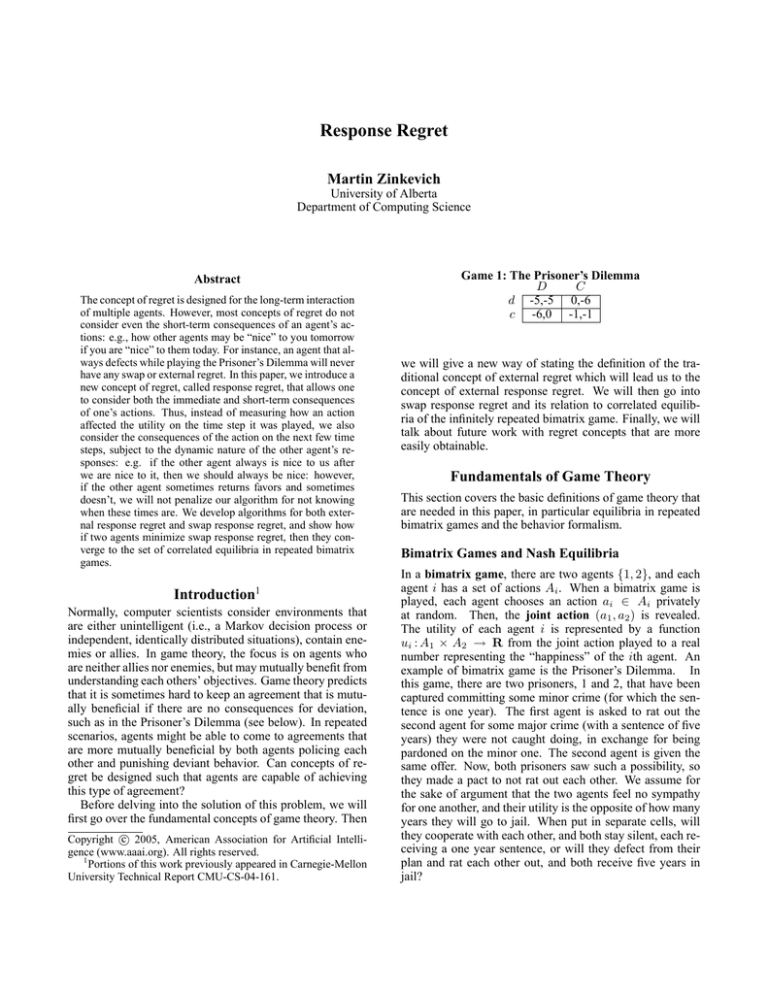
Game 1: The Prisoner’s Dilemma
D
C
d -5,-5 0,-6
c -6,0 -1,-1
we will give a new way of stating the definition of the traditional concept of external regret which will lead us to the
concept of external response regret. We will then go into
swap response regret and its relation to correlated equilibria of the infinitely repeated bimatrix game. Finally, we will
talk about future work with regret concepts that are more
easily obtainable.
Fundamentals of Game Theory
This section covers the basic definitions of game theory that
are needed in this paper, in particular equilibria in repeated
bimatrix games and the behavior formalism.
Bimatrix Games and Nash Equilibria
In a bimatrix game, there are two agents {1, 2}, and each
agent i has a set of actions Ai . When a bimatrix game is
played, each agent chooses an action ai ∈ Ai privately
at random. Then, the joint action (a1 , a2 ) is revealed.
The utility of each agent i is represented by a function
ui : A1 × A2 → R from the joint action played to a real
number representing the “happiness” of the ith agent. An
example of bimatrix game is the Prisoner’s Dilemma. In
this game, there are two prisoners, 1 and 2, that have been
captured committing some minor crime (for which the sentence is one year). The first agent is asked to rat out the
second agent for some major crime (with a sentence of five
years) they were not caught doing, in exchange for being
pardoned on the minor one. The second agent is given the
same offer. Now, both prisoners saw such a possibility, so
they made a pact to not rat out each other. We assume for
the sake of argument that the two agents feel no sympathy
for one another, and their utility is the opposite of how many
years they will go to jail. When put in separate cells, will
they cooperate with each other, and both stay silent, each receiving a one year sentence, or will they defect from their
plan and rat each other out, and both receive five years in
jail?
Game 2: Shapley’s Game
R
P
S
r 0,0 0,1 1,0
p 1,0 0,0 0,1
s 0,1 1,0 0,0
agent to choose an action uniformly at random from all its
actions. Finally, for each agent i define:
kui k =
max
(a1 ,a2 )∈A1 ×A2
ui (a1 , a2 )−
min
(a1 ,a2 )∈A1 ×A2
ui (a1 , a2 ).
Correlated Equilibria
The first agent has two actions {d, c}, either (d)efect
or (c)ooperate, indicated on the left side of the table (see
Game 1). The second agent has two options, either (D)efect
or (C)ooperate, indicated on the top of the table. In each
entry of the table is a possible outcome. For instance, if
the first agent (d)efects and the second agent (C)ooperates,
then the first agent receives a utility of u1 (d, C) = 0 (does
not go to jail) and the second agent receives a utility of
u2 (d, C) = −6 (goes to jail for both crimes). This is indicated by the pair 0, −6 in the top right entry of the table.
Now, consider this from the perspective of the first agent:
since the actions of both agents are simultaneous, his action cannot affect the action of the second agent, so the first
agent should assume that the second agent’s action is fixed.
If the second agent will defect, then the first agent achieves
u1 (d, D) = −5 if it defects and u1 (c, D) = −6 if it cooperates. Thus, the first agent would be happier defecting
if the second agent defected. Similarly, if the second agent
will cooperate, then u1 (d, C) > u1 (c, C). Therefore, the
first agent is happier defecting regardless of what happens.
Similarly, the second agent is happier defecting regardless
of what happens. The pair, (d, D) is called a Nash equilibrium, because given the strategy (plan of action, possibly involving randomness) of one agent, the strategy of the
other agent maximizes expected utility. It is often argued
that a Nash equilibrium is the only way that two rational
agents would play.
Sometimes, there is no pair of deterministic actions that
are a Nash equilibrium. Shapley’s Game (Game 2) is like
“Rock-Paper-Scissors”, except if an agent loses it receives
the same utility as if it had tied.
For any set S, define ∆(S) to be the set of all probabilities
over S. For a distribution D and a boolean predicate P , we
use the notation Prx∈D [P (x)] to indicate the probability that
P (x) is true given that x was selected from D, and D(x) to
be the probability of x in the distribution D. An agent i
may use a mixed strategy βi ∈ ∆(Ai ), where it plays an
action at random according to a distribution. βi (ai ) is the
probability of choosing ai while using βi . Define:
X
ui (β1 , β2 ) =
β1 (a1 )β2 (a2 )ui (a1 , a2 ).
a1 ∈A1 ,a2 ∈A2
It is known (Nas50) that for any bimatrix game, there exists
a Nash equilibrium (β1∗ , β2∗ ) ∈ ∆(A1 ) × ∆(A2 ) such that:
u1 (β1∗ , β2∗ ) =
u2 (β1∗ , β2∗ ) =
max
u1 (β1 , β2∗ )
max
u2 (β1∗ , β2 ).
β1 ∈∆(A1 )
β2 ∈∆(A2 )
In other words, given the strategy of one agent, the other
agent cannot improve its expected utility by changing its
strategy. A Nash equilibrium for Shapley’s Game is for each
Sometimes, when dividing chores, or deciding who has to
perform some unpleasant task, people will “draw straws”:
that is, they each choose a straw from a fist, and whoever
gets the shortest straw has to perform the task. Or, they
might draw pieces of paper from a hat. Sometimes such an
agreement may be a priori better for all agents than fighting,
or being disorganized, et cetera.
For instance, in Shapley’s game, the expected utility of
each agent in a Nash equilibrium is 1/3. It would be better
if the two agents avoided “ties”. One way to do this might
be for one agent to play paper, and the other agent to play
scissors. They draw straws, and whoever draws the shortest
straw plays paper.
Unfortunately, this agreement is somewhat flawed. If the
second agent draws the shortest straw, and believes the first
agent would play (s)cissors, why wouldn’t the second agent
play (R)ock? Thus, such an agreement is not self-enforcing,
because the agent who draws the shortest straw isn’t motivated to comply with the agreement.
Imagine that instead of this public randomness, or the independent private randomness inherent in mixed strategy
Nash equilibria, what if one had a source of dependent private randomness. For example, imagine that a referee, a
third impartial agent, has a bag with six balls, labeled (r, P ),
(r, S), (p, R),(p, S),(s, R), and (s, P ). All the agents know
the six balls in the bag. The referee now draws a ball uniformly at random from the bag. It then privately informs the
first agent of the first element of the pair on the ball and the
second agent of the second element of the pair on the ball.
Observe that the difference between this situation and the
one before is that if the first agent is told to play (r)ock, then
with equal probability the second agent will have been told
to play (S)cissors or (P)aper. Thus, the first agent can do no
better than play the action it has been told to play. Observe
that if both agents play as they are told, then both agents will
have an expected utility of 21 .
In general, a correlated equilibrium is a joint distribution D ∈ ∆(A1 × A2 ) over the actions of the agents. For
any a∗1 ∈ A1 on which D has positive probability, for any
a∗2 ∈ A2 on which D has positive probability:
X
X
D(a∗1 , a2 )u1 (a∗1 , a2 ) = max
D(a∗1 , a2 )u1 (a1 , a2 )
a2 ∈A2
a1 ∈A1
a2 ∈A2
X
X
D(a1 , a∗2 )u2 (a1 , a∗2 ) = max
D(a1 , a∗2 )u2 (a1 , a2 ).
a1 ∈A1
a2 ∈A2
a1 ∈A1
(1)
In other words, if D is the distribution from which the referee draws a joint action, then given that one agent chooses
the action recommended by the referee, the other agent can
do no better than choose the action recommended by the
referee. An -correlated equilibrium is a distribution D
where Equation 1 almost holds, i.e.:
X
D(a∗1 , a2 )u1 (a∗1 , a2 ) + a2 ∈A2
> max
X
D(a∗1 , a2 )u1 (a1 , a2 )
a1 ∈A1
a2 ∈A2
agent i is a function σi :H → ∆(Ai ), a function from the
history observed to a strategy to play on the next time step.
In order to consider Nash equilibria in repeated bimatrix
games, we have to define the distribution over histories when
two agents play a repeated bimatrix game. Define h(t) to be
the first t joint actions of history h. ht,i is the action chosen
in the tth time step by agent i. The probability of σi playing
its part of history h ∈ H is:
X
D(a1 , a∗2 )u2 (a1 , a∗2 ) + a1 ∈A1
Pσi (h) =
> max
X
D(a1 , a∗2 )u2 (a1 , a2 ).
a2 ∈A2
a1 ∈A1
Repeated Bimatrix Games
Many people find the Nash equilibrium of the Prisoner’s
Dilemma unsettling. For instance, one could imagine two
nations in the grips of a nuclear arms race. Each knows that
if it obliterated the other nation, it would be marginally safer.
Each would like to strike back if it knew it would be struck.
However, the US and the USSR co-existed in such a precarious position for decades without annihilating each other. Is
there something wrong with the above analysis?
Observe that to cooperate in the Prisoner’s Dilemma is a
strictly dominated action: that is, regardless of the strategy
of the other agent, cooperating never maximizes an agent’s
expected utility. This implies that cooperating is not in any
Nash equilibrium or in any correlated equilibrium.
However, sometimes a situation can be better modeled as
a repeated bimatrix game: that is, two agents face each
other in the same bimatrix game an infinite number of times.
For instance, suppose that the US knows that the USSR will
retaliate against any nuclear strike today with a strike of its
own tomorrow. Also, the US believes there is a high probability that the USSR will not strike tomorrow unless the US
strikes today. Thus, it is now in the best interest of the US
not to strike today.
Each time a bimatrix game is played is called a time step.
Formally, one can consider the events in a bimatrix game to
form an infinite history h ∈ H ∞ , an infinite sequence of
joint actions. Define ht to be the tth joint action of the history h. In a discounted repeated bimatrix game, one has
a discount factor γ ∈ [0, 1], that can sometimes be considered the probability of continuing to the next time step, or
as a simple cognitive discounting of rewards that will not be
received for some time. Given a discount factor γ ∈ [0, 1]
and a history h ∈ h∞ , the utility of agent i is:
uγi (h) =
∞
X
γ t−1 ui (ht ).
t=1
The state of the repeated bimatrix game after t time steps
can beS
represented by a finite history h ∈ H t = (A1 × A2 )t .
∞
H = t=0 H t is the set of all finite histories, including ∅,
the history of length 0. |h| is the length of history h.
The most important aspect of repeated bimatrix games is
that both agents remember the entire history of joint actions
up until the last game played and can have their strategy in
the current bimatrix game depend upon it. A behavior for
|h|
Y
σi (h(t − 1))(ht,i ).
t=1
In other words, the probability that at each time step t, given
the history up until that point, agent i would have chosen
the action ht,i . The probability that the game begins with
h when the behaviors σ1 and σ2 are used is Pσ1 ,σ2 (h) =
Pσ1 (h)Pσ2 (h). Define PσT1 ,σ2 ∈ ∆(H T ) to be the associated probability distribution. The principle can be extended
to infinite histories, such that µσ1 ,σ2 is the measure over
infinite histories when σ1 and σ2 are played, where for all
h0 ∈ H:
µσ1 ,σ2 ({h ∈ H ∞ : h(|h0 |) = h0 }) = Pσ1 ,σ2 (h0 ).
h(σ1 , σ2 ) is a random variable indicating the history played.
Thus, the expected utility of agent i when two agents using
the behaviors σ1 and σ2 play each other is:
uγi (σ1 , σ2 ) = E[uγi (h(σ1 , σ2 ))].
Define Σi to be the set of all behaviors for agent i. A Nash
equilibrium is a pair of behaviors (σ1∗ , σ2∗ ), such that:
uγ1 (σ1∗ , σ2∗ ) = max uγ1 (σ1 , σ2∗ ).
σ1 ∈Σ1
uγ2 (σ1∗ , σ2∗ ) = max uγ2 (σ1∗ , σ2 ).
σ2 ∈Σ2
It is interesting to note that if (β1∗ , β2∗ ) is a Nash equilibrium
for a single stage of the repeated bimatrix game then the
behaviors that always use β1∗ and β2∗ are a Nash equilibrium
for the whole repeated bimatrix game. However, there can
also be more complicated Nash equilibria that may be more
beneficial for all of the agents.
Equilibria in Repeated Bimatrix Games
Assume that we are playing a discounted repeated Prisoner’s
Dilemma with a discount factor of γ = 2/3. Suppose that
the second agent has the following strategy (called a grimtrigger (OR94, p. 141) behavior):
1. If the other agent has never defected, cooperate.
2. Otherwise, defect.
This is a behavior for the second agent that can be represented as a function σ2 : H → ∆(A2 ). What should the
first agent do? If the first agent always cooperates, then it
receives a utility of −3. If the first agent defects on a time
step, then after that time step it should always defect. Thus,
it will receive −1 on each time step before it defects, 0 on
the first time step it defects, and −5 after that. If the first
time step it defects on is t, then it will receive a utility of:
Now, if the omniscient builder builds a robot to maximize its
expected utility, this becomes the external response regret:
t−2 !
t−1
2
2
(−1) 1 + . . . +
+ (0)
3
3
!
t t+1
2
2
+ (−5)
+
+ ... .
3
3
1 X
(u1 (a∗1 , ht,2 ) − u1 (ht )) .
max
a∗
1 ∈A1 |h|
t=1
This reduces to:
−3 − 7
t−1
2
.
3
This approaches −3 as t approaches infinity. Thus, it is better never to defect, and any behavior for the first agent that
never defects if the second agent always cooperates is a best
response to the grim-trigger behavior. The grim-trigger behavior is therefore a best-response to itself (an equilibrium).
When both agents use a behavior that always defects, their
discounted utilities are both −15. When they both use the
grim-trigger behaviors, they always cooperate and receive a
discounted utility of −3. Thus, by considering equilibria of
the repeated game, one can perform better.
Another equilibrium when γ = 32 is that both agents play
tit-for-tat: each agent cooperates on the first round, and for
every round thereafter an agent cooperates if and only if the
other agent cooperated on the previous round. Observe that
defecting instead of cooperating will increase the immediate
reward by 1 but will decrease the reward at the next time step
by 5, making it unwise to deviate from this equilibrium.
Is it possible that some learning algorithm exists that can
converge to always cooperating if the other agent is playing
tit-for-tat? We will talk about two more general guarantees
for learning algorithms that will both imply convergence to
always cooperating in tit-for-tat.
Traditional Regret and the Omniscient Builder
Consider the following formulation of traditional external
regret. We want to build a good behavior σ1 :H → ∆(A1 )
for our agent to play against some agent playing σ2 :H →
A2 , a deterministic behavior. We compare ourselves to an
omniscient builder. The omniscient builder observes σ1 and
σ2 play for T time steps and generate a history h ∈ H T . The
builder constructs a robot that can play one action a∗1 ∈ A1 .
Now, after its construction, the robot is placed uniformly at
random at some point in the history h. It plays for one time
step and compares its performance on that time step to that
of the first agent. Thus, if the robot is placed at time t, the
robot chooses the action a∗1 and the second agent chooses the
action ht,2 . Thus, the robot receives a utility of u1 (a∗1 , ht,2 ),
and the first agent receives a utility of u1 (ht ) on the same
time step. Thus, the expected (with respect to t) difference
is:
|h|
1 X
(u1 (a∗1 , ht,2 ) −u1 (ht )) .
|h| t=1
|h|
(2)
In other words, the builder knows the history, but not when
in the history the robot will play. This is the traditional external regret. Now, in the prisoner’s dilemma, such a robot
would always want to defect. This is because even though
the robot is dropped into a repeated game, it only plays one
time step, and never sees the consequences of its actions on
later time steps. Can we design a concept of regret where all
consequences of an action are considered?
Secondly, we can consider the traditional swap regret.
Imagine the omniscient agent builds a robot that, when it
arrives at a particular point in time, gets to see what the first
agent did before it makes its choice. Therefore, the program
of the robot is a function φ : A1 → A1 , and the expected
utility of the robot if it lands at time t is u1 (φ(ht,1 ), ht,2 ).
Define Φ1 = (A1 )A1 to be the set of all functions from A1
to A1 . Then the traditional swap regret is:
|h|
max
φ∈Φ1
1 X
(u1 (φ(ht,1 ), ht,2 ) − u1 (ht )) .
|h| t=1
(3)
We construct the empirical frequency of joint actions
of h ∈ H from the process of selecting a joint action uniformly at random from a history. The following is immediate from the definition of swap regret.
Theorem 1 If both agents have a swap regret less than on
history h, then the empirical frequency of joint actions is an
-correlated equilibrium.
Motivation for Response Regret
In a repeated bimatrix game, if the first agent uses a traditional no-external-regret behavior, then it considers how
well it could have done with a fixed action assuming that the
actions of the second agent are fixed. For instance, consider
the Prisoner’s Dilemma. In this game, if the first agent always defects, and the second agent cooperates on the first
time step and then always defects, then the first agent has
zero external regret.
Observe that the above history could be generated if the
second agent was playing tit-for-tat: always playing what
the first agent played on the time step before. And, if the second agent was playing tit-for-tat, the first agent could have
done significantly better by always cooperating. However,
traditional external regret does not measure this regret, and
in fact if both agents always cooperate, the first agent will
have a positive external regret.
To handle such issues, we introduce response regret. Response regret is a compromise between doing what is optimal given the other agent’s behavior (which is impossible
without knowing the other agent’s behavior in advance) and
doing as well as the best from some class of functions given
the second agent is unaffected by the first agent’s actions.
This is similar to research where one considers how well
one could do if the world were a finite state automata. Response regret basically considers the short-term effects of
any actions that an agent makes.
This brings up an important aspect of traditional noexternal-regret algorithms. In the Prisoner’s Dilemma, they
will almost surely converge to almost always defecting. Can
the concept of regret be modified to allow both agents to
cooperate without having regret?2
This paper will also discuss convergence of “the average
joint behavior” to the set of correlated equilibria if swap response regret is minimized, similar to (FV97) observing the
empirical frequency distribution converging to the set of correlated equilibria of the bimatrix game, but different in that
we discuss convergence to correlated equilibria of the repeated game.
External Response Regret
In this section, we introduce external response regret. We
show how it is a natural extension of traditional external regret when we think about traditional external regret as playing against a robot built by an omniscient builder in a trial.
We show an example of how two situations with the same
history but different behaviors for the second agent can have
drastically different response regret for the first agent. We
also show how, even if the first agent and the robot (see below) use the same behavior, zero response regret is not guaranteed.
In external response regret, when the robot is placed at
a random point in the history, we have the robot play for
a longer period of time, which we will call a trial. Now
the omniscient builder constructs a robot with a behavior
σ1∗ :H → A1 . The robot is again placed at some time step
t chosen uniformly at random. After each time it plays a
time step, a coin is flipped. With a probability of γ, it plays
another time step, unless time step |h| has been played (the
trial cannot last past the end of the observed history).
Define h(t) to be the first t joint actions of a history h, and
define σ2,h (h0 ) = σ2 (h ◦ h0 ). Thus, if the robot is placed
at time step t, then it will observe a behavior of σ2,h(t−1) .
Define the discounted utility of the ith agent for T time steps
playing h to be:
uγ,T
i (h) =
T
X
γ t−1 ui (ht ).
step t is:
γ,(|h|−t)+1
u1
(σ1∗ , σ2,h(t−1) ).
Thus, this is the utility of playing from time step t to |h|
with a discount factor of γ assuming the second agent begins
at t with the same behavior that it was using before. The
expected difference between the performance of the robot
and the performance of the first agent in a trial is:
|h|
1 X γ,(|h|−t)+1 ∗
u
(σ1 , σ2,h(t−1) )
|h| t=1 1
γ,(|h|−t)+1
−u1
(ht , ht+1 , . . . , h|h| ) .
Define Σ0i to be the set of all deterministic behaviors for the
ith agent. When the omniscient builder designs the robot to
maximize the robot’s expected utility, the expected difference on a trial becomes:
|h|
Rext,γ (h, σ2 ) = max
∗
0
σ1 ∈Σ1
1 X
|h| t=1
γ,(|h|−t)+1
u1
(σ1∗ , σ2,h(t−1) )
γ,(|h|−t)+1
−u1
(ht , ht+1 , . . . , h|h| ) .
This is the external response regret: the expected difference in utility in a trial between the omniscient builder’s
robot and the first agent. Examples of this quantity in certain
scenarios follow in the next section. Importantly, we show
later that external response regret can be estimated in some
cases, but it cannot be not known exactly without knowing
σ2 .
Finally, given a repeated bimatrix game (u and A), given a
γ > 0, we define a behavior σ1 : H → ∆(A1 ) to minimize
external response regret if for every > 0, there exists a
T > 0 such that for all σ2 : H → A1 , it is the case that:
P (∃t > T, Rext,γ (h(σ1 , σ2 )(t), σ2 ) > ) < .
Theorem 2 For any repeated bimatrix game, for any γ >
0, there exists a behavior that minimizes external response
regret.
For a proof, see (Zin04).
t=1
uγ,T
i (σ1 , σ2 )
Define
= E[uγ,T
i (h(σ1 , σ2 ))]. Thus, the expected utility of the robot in a trial given it begins at time
2
An earlier algorithm (dFM03) does almost as well as the best
expert even taking into account the actions of the other agent, but
only if the environment is flexible: effectively, at least for the experts used, the environment is “forgiving” and one can recover from
any mistake in the past. Our guarantees hold even if the environment is inflexible, and our measure of regret itself takes into account the flexibility of the environment. Also, (BBV04) extend the
concept of round to include a far longer period of time: this allows
the agents to observe some of the consequences of their actions in
some real scenarios, but does not address the theoretical problem
(even still, the agents do not observe how their actions now affect
the next round).
Measuring What Could Have Been
Consider the following history h: the first agent σ1 always
defects for one hundred time steps. The second agent cooperated on the first time step, and always defected thereafter.
Did the first agent choose a reasonable behavior?
Now, from the perspective of traditional external regret,
this is a very reasonable behavior: a robot dropped to play
for one time step would always defect, and thus given the
above history, the traditional external regret would be zero.
However, the external response regret of the first agent in
this scenario would depend on how the second agent would
have responded if the first agent had cooperated. For instance, the second could have been playing tit-for-tat, grimtrigger, or could have been oblivious to any actions of the
first agent. In a tit-for-tat behavior, one always plays the
action the other agent played on the last time step (starting with cooperate on the first time step). The difference
between tit-for-tat and a grim-trigger behavior is that the
tit-for-tat behavior is “forgiving”. Observe that the second
agent could have played either behavior and generated h.
However, Rext,2/3 (h, GRIM ) and Rext,2/3 (h, T F T ) are
quite different, as we show below. Roughly, the reason is
the first agent was doomed from the beginning of the second
time step playing grim trigger, but when playing tit-for-tat,
the first agent could have improved its situation at any time
up until the very end.
If the first agent was playing against grim-trigger, then
it could have conceivably done much better from the first
time step. However, given its behavior on the first time step,
it could have done no better than it did. The omniscient
builder would design a robot that always defects in this scenario (i.e., behave the same as the first agent), and therefore
the first agent would not have any external response regret.
The same would be the case if the second agent was completely oblivious to the first agent.
If the first agent was playing against tit-for-tat, then it
could have improved its outcome at any time by playing cooperate. The omniscient builder knows this and designs a
robot that cooperates for 99 time steps, and then defects.3
The first time step that the robot plays, it does 1 worse than
σ1 . However, on second and later time steps, the second
agent will cooperate with the robot, and thus the robot will
have four more utility than σ1 on later time steps. The average trial lasts about 3 time steps,4 so the external response
regret is about 7.5
Now, observe that it is impossible for the first agent to
compute its own response regret during the game. This is
similar to the situation in (ACBFS02), where they consider
a traditional regret setting where one does not know what
the outcome of the other actions would have been.
behavior of the algorithm after every history and show the
results to the omniscient builder before we begin.
Now, in order to formally think of how the robot will play,
we have to extend the concept of a “behavior” to include a
“suggestion” for the next action. Thus, an optimal agent has
a function of the form
∞
[
σ100: H t × (A1 )t+1 → A1 ,
t=0
i.e., its choice given the history of the actions its seen, the
suggestions its received in the past, and a suggestion of
what to do next. Define Σ001 to be the set of all such deterministic functions. As before, we can consider a history to be a function of three behaviors: the suggestion givingSfunction σ1 : H → A1 , the suggestion taking function
∞
σ100: t=0 H t × (A1 )t+1 → A1 , and a deterministic behavior
for the other agent σ2 :H → A1 . Defining it recursively, if
h0 = h(σ1 , σ100 , σ2 ), then:
h0t,1
= σ100 (h0 (t − 1),
h0t,2
{σ1 (h0 (0)), σ1 (h0 (1)), . . . , σ1 (h0 (t − 1))})
= σ2 (h0 (t − 1))
Thus, in order to decide what to do next, σ100 asks σ1 what
it would do. Then, σ100 takes the history and the suggestions of σ1 into account, and makes a decision. σ2 just
00
decides based on the history. Define uγ,k
1 (σ1 , σ1 , σ2 ) =
γ,k
00
u1 (h(σ1 , σ1 , σ2 )).
Given a deterministic behavior σ1 :H → A1 , a deterministic behavior σ2 :H → A2 , and a history h that they both
would play, then the swap response regret is:
|h|
Rint,γ (σ1 , σ2 , h) = max
00
00
σ1 ∈Σ1
Swap Response Regret
Traditional swap regret in a repeated bimatrix game can be
framed in the following way. First, an algorithm interacts
with an environment, and a history is observed. Then, an
omniscient builder, who knows the environment and the history played, builds a robot that is placed at a point uniformly
at random in the history, but doesn’t know which one. Before the robot acts, it observes the next action that the other
agent would have made, and then chooses an action. As with
the external version, swap response regret can be formed by
having the trial extend to another time step with a probability
γ. On this next step, the robot finds out what the algorithm
would have done in the next step, given the robot’s original
deviation. Formally, we can imagine that we simulate the
3
This defection on the one hundredth time step is because it
is certain that the trial will end. However,
of the trial
the chance−20
1
2 99
lasting one hundred time steps is 100
≈ 4 × 10
.
3
100
4
Precisely, 2.98 + 0.02 23
≈ 2.98 ± 5 × 10−20 .
5
Taking into account the exact average trial length and the defection of the robot on its hundredth time step, the exact external
100
response regret is 6.92 + 0.095 23
≈ 6.92 ± 2 × 10−19 .
γ,(t−|h|)+1
u1
1 X
|h| t=1
σ1,h(t−1) , σ100 , σ2,h(t−1)
γ,(t−|h|)+1
−u1
ht , . . . , h|h|
.
Given this definition, we can define what we mean by
swap response regret. In particular, a behavior σ1 : H →
∆(A1 ) is said to minimize swap response regret, if for every > 0 there exists a T such that, for every σ2:H → A2 :
Pσ10 ∈σ1 (∃t > T, Rint,γ (σ10 , σ2 , h(σ10 , σ2 )(t)) > ) < .
Here, we have interpreted σ1 to be a distribution over behaviors of the form σ10 :H → A1 .
Theorem 3 For every game, for every γ > 0, there exists a
behavior that minimizes swap response regret.
Let us discuss Theorem 1 further. A correlated equilibrium (with rational probabilities) can be represented in the
following way. Imagine a referee has a bag of balls, and
each ball is labeled with a joint action. Before it begins, the
referee shows the bag to both agents. It then privately selects
a ball uniformly at random, and whispers in each agent’s ear
its part of the joint action. The interesting thing is that each
agent, given what they know about the balls in the bag, and
the fact that they know the referee will drawn one at random and read it accurately, they can do no better than use
the action the referee whispers in its ear. An -correlated
equilibrium can be represented in the same way, except that
the agents can improve by no more than by choosing some
other action other than the one whispered by the referee.
The sense in which the two agents minimizing swap regret
converge is as follows: imagine two agents played a history
finite history h. A referee has a bag of |h| balls: the ith ball
is labeled hi . According to the above procedure, the balls
in the bag represent an -correlated equilibrium, and as the
history grows longer, if the swap regret gets lower, gets
smaller.
Now, this can be extended to correlated equilibria of repeated games as well, and there are several different possibilities. Imagine now that instead of having joint actions,
each ball had an deterministic behavior for each action.
Now, instead of telling each agent its entire deterministic
behavior, the referee only tells each agent its next move. If
neither agent could do better than listen to the referee, the
distribution over deterministic behaviors is a correlated equilibrium. If either couldn’t do more than better, then it is an
-correlated equilibrium.
Imagine that the first agent acts according to σ1:H → A1 ,
the second agent acts according to σ2 : H → A2 , and the
history observed is h. Now, imagine that the referee has |h|
balls, and writes (σ1,h(i) , σ2,h(i) ) on the ith ball. As we argue below, this distribution would converge to a correlated
equilibrium of the repeated game if both agents are minimizing swap response regret.
Observe that the actions of each agent can be considered
to be the recommendations of the referee. If two algorithms
A and B are placed at a point chosen uniformly at random in
a history generated by two algorithms C and D minimizing
swap response regret, then neither A nor B can do much
better than simply doing what either C or D did.
Theorem 4 If two agents minimizing swap response regret
play against each other and generate h, then for any > 0,
with high probability, given a long enough history h, a joint
distribution over behaviors determined by their behaviors
and the history of play h in the above manner is an correlated equilibrium.
Observe that this correlated equilibrium is not necessarily subgame perfect. For example, imagine the following
variant of tit-for-tat in the Prisoner’s Dilemma: if the other
agent cooperated the last time step, then cooperate, otherwise defect 9/10 of the time. Now, if the agents both use
this behavior, then it is not in either’s best interest to ever
defect: the retaliation makes it not worth it. However, since
this is the case, they will almost never defect, and thus they
will almost never need to retaliate against a defection. Swap
response regret is minimized, and yet a correlated equilibrium that is not subgame perfect is reached.
Thus, it is an open question whether there exists an
achievable variant of swap response regret where if all
agents use this variant, they will converge to a subgame perfect correlated equilibrium.
Future Work
The main problem with response regret is that convergence
is slow. Therefore, we also plan to introduce other concepts
of regret where convergence is faster.
Program Regret
Suppose that you were not concerned with the performance
of the algorithm with respect to an arbitrary behavior, but
merely one from a small class of programs. For instance,
in the Prisoner’s Dilemma, it might be useful to compare
one’s performance to the four behaviors of always defecting,
always cooperating, grim trigger, and tit-for-tat.
Suggestion Regret
Imagine that there is both an agent and an advisor: the agent
is in some arbitrary world (e.g.a repeated bimatrix game,
a partially observable Markov decision process, a Markov
game), and is making observations and taking actions. However, the behavior of the agent is dependent upon the suggestions received by the advisor. Instead of considering the
quality of the behavior of the agent, we consider the quality of the suggestions of the advisor, which we measure in
a way similar to response regret. Again, we have an omniscient builder, who designs a robot to replace the advisor
instead of the agent. The possible programs the omniscient
builder can use is limited to those that are silent after the
first round (but can make any suggestion on the first round).
This model has very many similarities to the program regret
model, but it emphasizes the fact that the agent can respond
in any way whatsoever to the suggestions.
Conclusion
Traditional regret minimization focuses on the immediate
utility obtained by an agent. Response regret considers both
immediate and short-term effects of the actions of an agent.
We have demonstrated that it can allow cooperative behavior in the repeated prisoner’s dilemma. Moreover, swap response regret converges to a correlated equilibrium of the
repeated bimatrix game, which are more desirable in many
games.
References
P. Auer, N. Cesa-Bianchi, Y. Freund, and R. Schapire. The
nonstochastic multiarmed bandit problem. SIAM Journal
on Computing, 32(1):48–77, 2002.
M. Bowling, B. Browning, and M. Veloso. Plays as effective multiagent plans enabling opponent-adaptive play
selection. In Proceedings of the Fourteenth International
Conference on Automated Planning and Scheduling, pages
376–383, 2004.
D. de Farias and N. Meggido. How to combine expert (or
novice) advice when actions impact the environment. In
Advances in Neural Information Processing Systems 17,
2003.
D. Foster and R. Vohra. Calibrated learning and correlated
equilibrium. Games and Economic Behavior, 21(1):40–55,
1997.
J. Nash. Equilibrium points in n-person games. Proceedings of the National Academy of Sciences, 36:48–49, 1950.
M. Osborne and A. Rubinstein. A Course in Game Theory.
The MIT Press, 1994.
M. Zinkevich. Theoretical Guarantees for Algorithms in
Multiagent Settings. PhD thesis, Carnegie Mellon University, August 2004.