From: AAAI Technical Report FS-02-01. Compilation copyright © 2002, AAAI (www.aaai.org). All rights reserved.
Possibility Theory in the Management of Chance Discovery
Ronald R. Yager
Machine Intelligence Institute
Iona College
New Rochelle, NY 10801
E-mail: yager@panix.com
Introduction
The purpose this work is to discuss and investigate
the potential role of possibility theory [1-4] and other
non-standard uncertainty calculi, such as the DempsterShafer theory [5, 6] of evidence, in the development of
a framework for the management of chance discovery.
Possibility theory provides a framework for the
representation and management of information about
uncertain situations. It is closely related to fuzzy set
theory. Possibility theory uses two dual measures,
called the possibility measure and certainty (necessity)
measure, to model available information about
uncertainty situations. As opposed to probability
theory. where the probability measure is additive, the
possibility measure involves Maxing of its elements
and the Certainty measure, which is the dual of the
possibility involves Mining of its elements. In
addition possibility theory is not as strongly constrained
by the law of the excluded middle allowing a more
flexible framework.
A particularly important feature of possibility
theory and these other non-standard calculi are their
ability to represent information that is not impossible.
Here we have a framework in which we are able to
manage outcomes that are not expressly denied although
never have occurred. Its close relationship with fuzzy
set theory makes it very suitable for the representation
of information about uncertainty that is not necessarily
of a random type. Here we shall focus on the issue of
decision in the face of possibility and other types of
uncertainty,
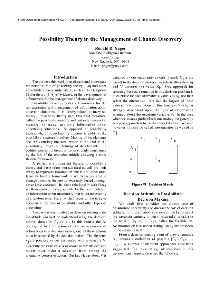
The basic issues involved in decision making under
incertitude can best be understood using the decision
matrix shown in figure #1. In this matrix the Ai
correspond to a collection of alternative courses of
action open to a decision maker, one of these actions
must be selected by the decision maker. The elements
x j are possible values associated with a variable V.
Generally the value of V is unknown before the decision
maker must make a selection from among the
alternative courses of action. Our knowledge about V is
captured by our uncertainty calculi. Finally Cij is the
payoff to the decision maker if he selects alternative Ai
and V assumes the value Xj . One approach for
selecting the best alternative in this decision problem is
to calculate for each alternative a value Val(Ai) and then
select the alternative that has the largest of these
values. The formulation of this function Val(Ai) is
strongly dependent upon the type of information
assumed about the uncertain variable V. In the case
when we assume probabilistic uncertainty the generally
accepted approach is to use the expected value. We note
however this can be called into question as we did in
[7].
x
x
x
1
j
n
A
A
1
i
C
ij
Am
Figure #1. Decision Matrix
Decision Attitude in Possibilistic
Decision Making
We shall first consider the classic case of
possibilistic uncertainty and discuss the role of decision
attitude. In this situation in which all we know about
the uncertain variable is that it must take its value in
the set X = {x1 , x2 , ..... xn }, called the feasible set.
No information is assumed distinguishing the prospects
of the elements in X.
From a decision making point of view alternative
A i induces a collection of possible [Ci1 , C i2 , ....,
C in ]. A number of different approaches have been
suggested for evaluating alternatives in this
environment. Among these are the following:
1). Pessimistic: Val(Ai) = Minj[C ij]
2). Optimistic: Val(Ai) = Maxj[C ij]
n
1
Cij
3). Average/neutral: Val(Ai) =
n
j =1
4). Arrow-Hurwicz Criteria:
Val(Ai) = a Maxi[Cij] + (1 - a) Mini[Cij] (for a[0, 1])
Each one of these can be seen as reflecting a particular
attitude on the part of the decision maker. For example,
in the first one the decision maker is essentially
displaying a pessimistic attitude, one in which he is
assuming that the worst of the possible outcomes will
occur. Thus we see that a significant aspect of these
methods is the centrality of the choice of decision
attitude in the process of valuating alternatives. Also,
quite clear in this situation is the subjectiveness of the
choice.
In [ 8 ] we provided for a unification and
generalization of these approaches to decision making.
The approach is based upon the OWA operator [9, 10].
We first describe the OWA operator.
An Ordered Weighted Averaging (OWA) operator
of degree n is a mapping FW : Rn Æ R which has an
associated vector weighting vector W, whose
components satisfy
W-1:. wj Π[0,1] for j = 1 to n
n
W-2:.
wj = 1
j =1
n
and where F w (a 1 , a2 , ......, an ) =
w j b j with bj
j =1
being the jth largest of the ai.
Essentially, the OWA operator involves a
reordering of the arguments, then a linear aggregation.
Thus if B is the vector of reordered arguments then we
can express this as
Fw( a1, a2, ......, an) = WT B,
it is the inner product of the weighting vector and the
vector of ordered arguments.
In [8] we suggested the use of the OWA operator as
a structure for providing a unification and generalization
of the decision making formalisms used in decision
making under possibilistic uncertainty. Assume Ai is a
decision alternative with payoff bag [Ci1 , Ci2 , ....,
Cin] then we suggested using Val(Ai) = FW (Ci1, Ci2,
...., Cin ) as the valuation of the alternative. By
appropriately selecting W we can obtain any of the
previously introduced evaluation functions.
Â
Â
Â
1). If W = W
where wj = 0 for j = 1 to n - 1 and
*
w n = 1, we get Val(Ai) = Minj[C ij], the pessimistic
decision maker.
2) If W = W*, where w1 = 1 and w = 0 for j = 2 to
j
n, we get Val(Ai) = Maxj[Cij] the optimistic decision
maker..
3).If W = WA , where wj = 1 for all j we get
n
n
1
Ci. the neutral decision maker
Val(Ai) = n
j =1
4) If W = WH, where w1 = a, wn = 1 - a and wj =
0 for j = 2 to n - 1 we get Val(Ai ) = aMax j [C ij ] +
(1 - a) Minj[Cij], the Arrow-Hurwicz criteria.
In [8] we referred to W as the attitudinal vector and
introduced a measure of optimism associated with a
n
given vector: a(W) = 1
w j (n - j). We note
n - 1 j =1
that a ( W * ) = 0, a ( W * ) = 1, a( W A ) = 0.5 and
Â
Â
a(W H ) = a
In addition to unifying the existing decision
making techniques, the introduction of the OWA
formalism provides for a generalization of the potential
means we have for evaluating alternatives. The
generalization introduced here is one in which by
selecting a W we get a valuation function. This of
course provides us with an infinite family of possible
valuation functions. It would be useful here to address
the issue of providing some direction for the process of
selecting an attitudinal vector W. The more deep our
understanding of the valuation methodology, the more
intelligently we can select the attitudinal vector W.
In [11] Yager suggested an interesting interpretation
of the valuation process. Noting that the elements in
the attitudinal vector W, as required by W-1 and W-2,
satisfy the properties of a probability distribution, they
lie in the unit interval and sum to one, he suggested
that the components in W can be interpreted as a kind of
subjective probabilities. In particular, he suggested that
wj can be interpreted as the decision maker's subjective
probability that the jth best outcome will occur. With
this interpretation, the pessimist is saying, since in this
case wn = 1, that the probability that the worst thing
will happen is one while the optimist is saying that the
probability that the best thing will happen is one.
Under this interpretation of the wj's, as these type of
probabilities and with bj being the jth best payoff, we
n
see then the evaluation Val(Ai) =
Â
bj wj is a kind of
j =1
expected value.
In order to use this OWA approach for valuating
alternatives, we need select an attitudinal vector W. A
number of approaches have be suggested for the
determination of the attitudinal vector W. Here we
describe one approach. In this approach, all that is
required of the decision maker is that they provide a
value a Π[0, 1] indicating their desired degree of
optimism. Using this value the weights for the
appropriate attitudinal vector can be obtained by solving
the following mathematical programming problem.
n
Maximize:
wj ln(wj)
j =1
Subject to:
1.w Π[0, 1]
j
n
2.
wj = 1
j =1
n
3. 1
wj (n - j) = a
n - 1 j =1
In the above we see that constraints 1 and 2 are the
basic constraints for the OWA vector. Constraint 3
assures us that the degree of optimism of the determined
vector satisfies our desired condition of a . The
objective function can be seen as one of maximizing the
entropy of the determined weights. This approach can
be seen as a generalization of the Arrow-Hurwicz criteria
[12]. In both approaches the decision maker supplies a
degree of optimism. In the Arrow-Hurwicz criteria, we
only allocate weight to the maximal and minimal
payoffs associated with an alternative. In this approach
the weight is distributed to all the payoffs associated
with the alternative being evaluated.
The following example illustrates the use of the
OWA operator.
Â
Â
Â
x1
x2
x3 x4
Example: A1
100
30
60 50
A2
70
60
50 80
Here
B1 =
100
80
60
and B2 = 70
50
30
60
50
are the ordered payoffs for alternatives A1 and A2
respectively. Let us look at different kinds of decision
makers.
(1)
W T = 1 1 0 0 , this is a strongly
2 2
optimistic decision maker. In this case
Val(A1) = 1 (100 + 60) = 80
2
Val(A2) = 1 (80 + 70) = 75
2
Here A1 is the preferred alternative..
(2) If WT = 0 0 1 1 , strongly pessimistic
2 2
decision maker. In this case
Val(A1) = 1 (50 + 30) = 40
2
Val(A2) = 1 (60 + 55) = 55
2
Here A2 is preferred.
(3)
For the neutral decision maker,
T
1
1
1 1 we get
W =
4 4 4 4
Val(A1) - 1 (100 + 60 + 50 + 30) = 60
4
Val(A2) = 1 (80 + 70 + 60 + 50) = 65
4
Here A is again preferred.
2
(4) If we consider a decision maker with a = 0.65
and use the weights obtained by solving the preceding
mathematical programming problem, we have
WT = 0.4 0.28 0.19 0.13
In this case
Val(A1 ) = (4)100 + (0.28)(60) + (0.19))50
+ (13)50 = 70.2
Val(A2 ) = (0.4)80 + (28)(70) + (0.19))60
+ (13)50 = 69.5
Decision Making with D-S Belief
Structures
We have considered decision making in situations
in which the information about the uncertain variable V
is possibilistic. The Dempster-Shafer belief structures
provides another uncertain knowledge representation.
We first provide a formal characterization of the
Dempster–Shafer belief structure.
A Dempster-Shafer belief structure defined on a set
X has an associated collection of subsets of X, Bj for
j = 1 to n, called focal elements and a mapping m
associating values with subsets of X,
m:2X Æ [0, 1]
such that:
n
1).
Â
m(Bj) = 1
j =1
2). m(A) = 0 for A not a focal element.
Two measures that are defined on these belief
structures, which we shall find useful, are the measure
of plausibility and belief. The plausibility measure Pl
is a mapping Pl: 2X Æ [0,1] defined as
Pl(A) =
Â
m(Bj).
all j s.t.
A « B jπ ∆
The measure of belief, Bel, is a mapping on subsets of
Xdefined by
Bel(A) =
Â
m(Bj)
all j s.t.
A Õ Bj
It can be shown that Bel(A) = 1 - Pl(A).
An important special case of belief structures are
called consonant belief structure in this case the focal
elements are nested, that is they can be indexed so that
B 1 Ã B 2 .... Ã B n . In this case the plausibility
measure has the special property that
Pl(E » F) = Max[Pl(E), Pl(F)]
A various semantics can be associated with the D-S
belief structure. We shall find the following semantics,
one very much in the spirit of random sets, useful for
our current interest, decision making under uncertainty.
Let V be a variable that takes its value in the set X.
Assume our knowledge about the value of this variable
is that it is determined at least in part by performance of
a biased random experiment. In this random experiment
the outcomes, rather being elements of X are subsets of
the space X. Furthermore, it is assumed that the actual
value of V must be an element of the set that is
determined by the random experiment. We let pj be the
probability that F j is the outcome subset of the
experiment. If we assign Fj = Bj and let m(Bj ) = pj
then we can represent this as a D-S belief structure.
Probabilistic uncertainty is a special case of this
structure in which the focal elements are singletons,
B j = {xj} and m(Bj) = pj, the probability of xj..The
possibilistic uncertainty previously discussed is a
special case of a belief structure, it is one in which
B1 = X and m(B1) = 1.
The next example is an illustration of a case in
which we have knowledge of an uncertain variable that
is not representable by the possibilistic or probability
model but is representable by the D-S belief structure.
Let V be a variable corresponding to interest rates
at some future date. Assume interest rates are
determined by the Federal Reserve Board. Assume that
the board is considering three policies: make interest
rates low, make interest rates high and not interfere with
interest rates. We believe that there is a 50% chance
that the first policy will be followed, 20% chance of the
second and a 30% chance of the third. We can represent
the information about the variable V, future interest
rates, as a belief structure in which B1 is the subset of
X, the set of interest rates, consisting of low interest
rates, B2 is the subset of X consisting of high interest
rates and B3 = X, any interest rate.
Given a D-S belief an issue of concern is the
determination of the probability that the value of V lies
in some subset A of X; Prob(A). Generally, because of
the type of uncertainty modeled by the D-S this value
can't be precisely obtained. The best we can do is to
find upper and lower bounds, Prob+(A) and Prob-(A)
such that
Prob-(A) £ Prob(A) £ Prob+(A)
It can be shown that these bounds are related to the
measures of of plausibility and belief introduced earlier,
in particular Prob+(A) = Pl(A) and Prob-(B) = Bel(A).
Using this D-S representation various types of the
knowledge can be represented for example the
knowledge that that Prob(A) ≥ a is representable by a
belief structure in which B1 = A and B2 = X and m(B1)
= a and m(B 2 ) = 1 - a. The knowledge that Prob(A)
= a is representable in this structure by a belief
structure in which B1 = A and B2 = A and where
m(B 1 ) = a and m(B 2 ) = 1 - a.
We shall now turn to the issue of decision making
in situations in which our knowledge about the
uncertain variable is represented by a D-S belief
structure.
Assume we have a decision problem where our
knowledge about the uncertain variable V is represented
by a belief structure with focal elements F1 , ...., Fq
with weighting function m. In [8] we suggested a
general approach to this decision problem based upon a
determination of a valuation Val(A i ) for each
alternative. The procedure used for the valuation of an
alternative is given in the following. In order to use
this approach the decision maker must provide a value
a Π[0, 1] corresponding to the degree of optimism
they want to use in the decision problem. This degree
of optimist will be used to generate attitudinal
weighting vectors using algorithm of the earlier section.
In the following we shall use Wa,r to indicate the
attitudinal vector of dimension r generated from this
algorithm based upon a degree of optimism. The
procedure evaluating alternative Ai is as follows:
1). For each focal element Fj calculate Val(Ai/j)
where Val(A i / j ) = (Wa ,n ) T Bj. H ere nj is the
j
cardinality of the focal set Fj , Bj is the n vector
consisting of the ordered payoffs that are associated with
the elements in Fj and the alternative Ai. (Val(Ai/j) is
an OWA aggregation with attitudinal vector Wa,n and
j
arguments Cik for all xk ΠFj).
2) Calculate Val(Ai) as the expected value of the
Val(Ai/j) that is
n
Val(Ai) =
Val(Ai/j) pj
j =1
here of course pj = m(Bj).
We see that in step one we used the possibilistic
technique and in step two we used the expected value
characteristic of probabilistic environment.
The following example illustrates the procedure
just described.
Example: Again we assume the following decision
matrix:
x1
x2
x3
x4
A1
100
60
70
50
A2
90
80
60
100
We assume knowledge of the uncertain variable V
is expressed by the following belief structure with three
focal elements: F1 = {x1 , x2 }, F2 = {x2 , x3 , x4 } ,
F 3 = {x 3 , x4 } where m(F1 ) = 0.5, m(F2 ) = 0.3 and
m(F3) = 0.2.
Here we shall assume our degree of optimism a =
0.75. Using our algorithm we obtain the following
attitudinal vectors for n = 2 and 3.
n = 2: w1 = 0.75
w2 = 0.25
Â
n=3
w1 = 0.62
w2 = 0.27 w3 = 0.11
For F1, F2, and F3 the collection of associated payoffs
are respectively [100, 60], [60, 70, 50] and [70, 50].
These result in following ordered payoff vectors:.
10
100
70
B1 =
B2 = 60
B3 =
60
50
50
Using this we get
Val(A1/1) = (100)(0.75) + (60)(0.25) = 90
Val(A1/2) = (70)(0.62) + (60)(0.27) + 50(0.11) =65.1
Val(A1/3) = (70)(0.75) + (50)(0.25) = 65
Finally,
3
Val(A1) =
Â
Val(A1/j) pj
j =1
= (90)(0.5) + (65.1)(0.3) + (65)(0.2) = 77.53
If we used a = 0.5 instead of 0.75 then for
n = 2: w1 = w2 = 1
2
n = 3: w1 = w2 = w3 = 1
3
In this case
Val(A1/1) = 1 (100 + 60) = 80
2
Val(A1/2) = 1 (60 + 70 + 50) = 60
3
Val(A1/3) = 1 (70 + 50) = 60
2
Here Val(A1) = (80)(0.5) + (60)(0.3) + (60)(0.2) = 70.
Notice the valuation for a = 0.5 is less then the case in
which we used a = 0.75 this is because it is more
pessimistic.
We can calculate Val(A2 ) in a similar manner,
however we shall not do this.
Graded Possibilistic Decision Making
Possibilistic uncertainty is often generated from
linguistic information. An example of this is the
statement "interest rates will be low." Here we obtain
as the set of possible interest rates all those considered
as low. With the introduction of Zadeh's work on fuzzy
sets [13] we have become much more aware of the fact
that concepts such as "low interest rates" rather than
being crisp and well bounded are imprecise and fuzzy.
In particular, the set of low interest rates rather than
being a crisp set is in reality a fuzzy subset. This
observation requires us to have to come to grips with
graded possibilistic information. In particular,
information about a variable V based on fuzzy subsets
induces a possibility distribution P [1] on the domain
of V where for each x in the domain P (x) Π[0, 1]
indicates the possibility that x is the value of the
variable V. We shall at this point not digress into the
theory of possibility, however we note that [3, 14]
provides a comprehensive introduction to the field.
Here we shall only consider the problem of decision
making with graded possibilities. Thus we shall
assume for each x ΠX there exists a value P(x) Π[0,
1] indicating the possibility that x is the value of V.
As with all cases of possibilistic decision making
we must provide some indication of the decision makers
attitude, here we shall assume a decision maker with
degree of optimism a. For notational simplicity we
shall use OWAa(G) to indicate the aggregation of the
elements in the set G using the attitudinal vector
generated by a degree of optimism a and dimension
equal to the cardinality of G.
In calculating Val(A i ) in this case of graded
possibilistic uncertainty rather then treating all
outcomes similarly we need give more weight to those
outcomes having larger grade of possibility. The
following is a procedure for evaluating Val(Ai) in this
environment of graded possibility
0. Determine the largest degree of possibility for
any element in the domain X of the uncertain variable
and denote this as Umax.
1. For each u Π[0, Um a x ] denote Fu as the
subset of X for which P(x) ≥ u. Fu are sometimes
called level sets.
2). For each Fu obtain the bag of associated
payoffs for the alternative being evaluated, Bu. Thus if
xk ΠFU then Cik is in the bag Bu.
3). Calculate Val(Ai/u) = OWA (Bu)
a
Umax
4) Val(Ai) = 1
OWAa du
Umax 0
The following example illustrates this approach.
Example: Assume the payoffs for alternative Ai is
x1
x2
x3
x4
100 60 70 50
A1
and we have the following information on graded
possibilities
P(x1) = 0.8, P(x2) = 0.3, P(x3) = 1, P(x4) = 0.5
In this case
Fu = {x1, x2, x3, x4}
u £ 0.3
Fu = {x1, x3, x4}
0.3< u £ 0.5
Fu = {x1, x3}
0.5 < u £ 0.8
Fu = {x3}
0.8 < u £ 1
and therefore,
Bu = {100, 60, 70, 50} u £ 0.3
Bu = {100, 70, 50}
0.3 < u £ 0.5
Bu = {100, 70}
0.5 < u £ 0.8
Bu = {70}
0.8 < u £ 1
For simplicity we shall assume a neutral decision
maker, a = 0.5. Thus at each level we take the average.
Val(A1/u) = 70
u £ 0.3
Val(A 1/u ) = 73.3
0.3 < u £ 0.5
Val(A1/u) = 85
0.5 < u £ 0.8
Val(A1/u) = 70
0.8 < u £ 1
1
Val(A1) =
A 1/u du = (70)(0.3) + (73.3)(0.2) +
0
(85)(0.3) + (70)(0.2) = 75.16
A natural extension here is to consider the cases in
which we have graded possibility in Dempster-Shafer
belief structures. In this case the focal elements rather
then being crisp subsets of the domain would be fuzzy
subsets of the domain. Here each focal element Fj
would induce a graded possibility distribution Pj on the
domain of the uncertain variable in which Pj(x) = Fj(x),
the membership grade of x in the fuzzy focal element.
The valuation process in this case would require that in
calculating Val(Ai/j), the valuation of the alternative
with respect to the jth focal element, we use the
procedure described in this section for graded
possibilistic decision making.
Conclusion
We believe that possibility theory and D-S theory
provide useful frameworks for the representation of
uncertainty in management chance discovery. Here we
have focused on the issue of decision making under
these types of uncertainty. We particularly noted the
importance of the role of decision attitude.
Reference
[1]. Zadeh, L. A., "Fuzzy sets as a basis for a theory of
possibility," Fuzzy Sets and Systems 1, 3-28, 1978.
[2]. Dubois, D. and Prade, H., Possibility Theory : An
Approach to Computerized Processing of Uncertainty,
Plenum Press: New York, 1988.
[3]. De Cooman, G., Ruan, D. and Kerre, E. E.,
Foundations and Applications of Possibility Theory,
World Scientific: Singapore, 1995.
[4]. Yager, R. R., "On the instantiation of possibility
distributions," Fuzzy Sets and Systems 128, 261-265,
2002.
[5]. Shafer, G., A Mathematical Theory of Evidence,
Princeton University Press: Princeton, N.J., 1976.
[6]. Yager, R. R., Kacprzyk, J. and Fedrizzi, M.,
Advances in the Dempster-Shafer Theory of Evidence,
John Wiley & Sons: New York, 1994.
[7]. Yager, R. R., "Fuzzy modeling for intelligent
decision making under uncertainty," IEEE Transactions
on Systems, Man and Cybernetics Part B: Cybernetics
30, 60-70, 2000.
[8]. Yager, R. R., "Decision making under DempsterShafer uncertainties," International Journal of General
Systems 20, 233-245, 1992.
[9]. Yager, R. R., "On ordered weighted averaging
aggregation operators in multi-criteria decision
making," IEEE Transactions on Systems, Man and
Cybernetics 18, 183-190, 1988.
[10]. Yager, R. R. and Kacprzyk, J., The Ordered
Weighted Averaging Operators: Theory and
Applications, Kluwer: Norwell, MA, 1997.
[11]. Yager, R. R., "On the inclusion of importances in
OWA aggregations," in The Ordered Weighted
Averaging Operators: Theory and Applications, edited
by Yager, R. R. and Kacprzyk, J., Kluwer Academic
Publishers: Norwell, MA, 41-59, 1997.
[12]. Arrow, K. J. and Hurwicz, L., "An optimality
criterion for decision making under ignorance," in
Uncertainty and Expectations in Economics, edited by
Carter, C. F. and Ford, J. L., Kelley: New Jersey,
1972.
[13]. Zadeh, L. A., "Fuzzy sets," Information and
Control 8, 338-353, 1965.
[14]. Klir, G. J. and Yuan, B., Fuzzy Sets and Fuzzy
Logic: Theory and Applications, Prentice Hall: Upper
Saddle River, NJ, 1995.