From: AAAI Technical Report FS-94-02. Compilation copyright © 1994, AAAI (www.aaai.org). All rights reserved.
Relevance Measures for Localized Partial
Networks
Evaluation
of Belief
Denise L. Draper
Department of Computer Science and Engineering
University of Washington, Seattle, WA98105
ddraper@cs,washington, edu
1
Introduction
Localized partial
evaluation (LPE) [Draper and
Hanks, 1994] is an algorithm for computing bounds
on the marginal probability of a variable in a belief
network. LPEaccomplishes this by considering information incrementally, attempting to find more relevant information first. In the following sections, we
briefly describe belief networks, the localized partial
evaluation algorithm, and then discuss how relevance
can be defined and used in LPE.
?
visit-to-asia./~~ng
= true
f~tubercul°sisz-~
~
lnng-canc~~..~
bronchitis
~..jCz shortness-of-breath
2
Belief
Networks
( ")X-ray
"
Belief networks (also called probabilistic networks,
Bayesian networks and causal networks) provide a way
of encoding knowledge about the probabilistic dependencies and independencies of a set of variables in some
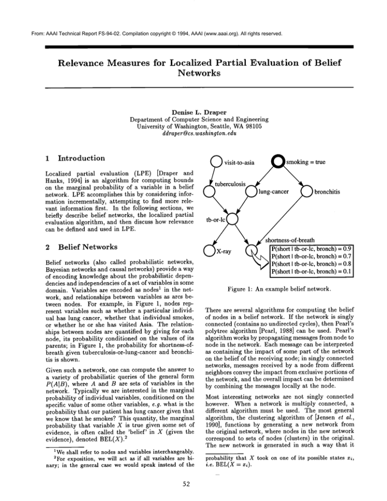
domain. Variables are encoded as nodes1 in the network, and relationships between variables as arcs between nodes. For example, in Figure 1, nodes represent variables such as whether a particular individual has lung cancer, whether that individual smokes,
or whether he or she has visited Asia. The relationships between nodes are quantified by giving for each
node, its probability conditioned on the values of its
parents; in Figure 1, the probability for shortness-ofbreath given tuberculosis-or-lung-cancer and bronchitis is shown.
Given such a network, one can compute the answer to
a variety of probabilistic queries of the general form
P(AIB), where A and B are sets of variables in the
network. Typically we are interested in the marginal
probability of individual variables, conditioned on the
specific value of someother variables, e.g. what is the
probability that our patient has lung cancer given that
we know that he smokes? This quantity, the marginal
probability that variable X is true given some set of
evidence, is often called the ’belief’ in X (given the
2evidence), denoted BEL(X).
1Weshall refer to nodes and variables interchangeably.
2For exposition, we will act as if all variables are binary; in the general case we wouldspeak instead of the
52
(" k~ [P(short I tb-or-!c, bronch)=
"~-~’~.,. [ P(short I tb-or-lc, bronch)=0.7
"~,~1P(short I tb-or-lc, bronch)=0.8
" [P(sbort
I tb-or-lc, bronch)=0.1
Figure 1: An example belief network.
There are several algorithms for computing the belief
of nodes in a belief network. If the network is singly
connected (contains no undirected cycles), then Pearl’s
polytree algorithm [Pearl, 1988] can be used. Pearl’s
algorithm works by propagating messages from node to
node in the network. Each message can be interpreted
as containing the impact of some part of the network
on the belief of the receiving node; in singly connected
networks, messages received by a node from different
neighbors convey the impact from exclusive portions of
the network, and the overall impact can be determined
by combining the messages locally at the node.
Most interesting networks are not singly connected
however. When a network is multiply connected, a
different algorithm must be used. The most general
algorithm, the clustering algorithm of [Jensen el al.,
1990], functions by generating a new network from
the original network, where nodes in the new network
correspond to sets of nodes (clusters) in the original.
The new network is generated in such a way that it
probability that X took on one of its possible states xi,
i.e. BEL(X= xi).
is singly connected, and thus messages may be propagated through the new network in a similar manner
to the singly connected case.
Pearl’s algorithm on a singly connected network is linear in the size of the network. Exact solutions to
multiply connected networks, however, are NP-hard
[Cooper, 1990]. Further, intractable cases are not perverse: such behavior is often encountered in networks
of realistic complexity. (Intuitively, the exponential
factor is associated with the loops in the network;
the more densely connected the network, the more intractable.)
Not surprisingly, considerable attention has been given
to finding approximate solutions to belief networks.
One approximation technique is Monte Carlo simulation of networks, which has also been shown to be
NP-hard [Dagum and Luby, 1993]. Other techniques
have included removing arcs from the network, e.g.
[Kjmrulff, 1993], and replacing very small probabilities by zero [Jensen and Andersen, 1990]. A particular
class of algorithms attempt to incrementally bound the
belief of a particular node by considering progressively
more information which has an impact on that node.
Twoexisting algorithms, [D’Ambrosio, 1993] [Poole,
1993], work (very roughly speaking) by factoring the
messages that are sent through the network, and incrementally considering the terms in the factors (bounding the possible impact of as-yet-unconsidered terms).
Localized partial evaluation functions by incrementally considering the impact that individual nodes have
on some target node.
3
Localized
Partial
Evaluation
At the top level, the Localized Partial Evaluation
(LPE) algorithm operates in an iterative fashion: the
user specifies a query node X, and LPE generates
an interval value Bl~L(X) that is guaranteed to contain BEL(X). Depending on the requirements
the user, this interval may or may not be adequate;
for example, the user may need to know whether or
not BEL(X) > 0.7, or might simply desire to know
BEL(X)to within +5%(i.e. the interval width must
be _< 0.1). If the user’s requirements are not met,
LPEcan be run again, producing a tighter interval
bound; in the limit, LPE will converge on the true
3point-valued BEL(X).
LPE produces the interval valued Bl~L(X) by considering only a subset of the nodes and arcs in the
network--conceptually, LPEignores parts of the network that are "too far away" from the query node
to have muchimpact on its belief value. Morespecifically, LPEoperates by first selecting a contiguous subset of the nodes and arcs in the network, called the
3Naturally, the user’s requirements can be encodedinto
a top-level routine whichrepeatedly invokes LPEuntil the
requirements are met.
53
active set, and then running a message-propagation
algorithm--such as Pearl’s algorithm--over only this
subset of the network. Messages which would have
been received over arcs not in the active set are replaced by interval-valued vacuous messages. The interval value of a vacuous message is a bound on the
value that the true message could take on if it were
to be computed. Inside the active set, messages are
computed in the normal fashion, but owing to the influence of vacuous messages, these internal messages
mayalso be (and generally are) interval-valued. Similarly the computedbelief of the query node is intervalvalued. WhenLPEis iterated, new nodes and arcs are
added to the active set, and vacuous messages which
had been used for the newly-added arcs are replaced
by their computedvalues (which will still generally be
interval-valued, because of the influence of still other
nodes and arcs not yet in the active set). The changed
messages are propagated, causing other messages to
be changed and recomputed (messages which are not
changed are cached and reused).
In a singly connected network, LPE operates as
an interval-valued extension to Pearl’s polytree algorithm. Wecan extend LPE to work with the clustering algorithm on multiply connected networks in one
of two ways: either the clustering algorithm can be
used to generate a singly connected clique network,
and LPEapplied to that network, or LPE can be used
to first select the active set from the original network,
and then (an interval-valued extension of) clustering
can be applied only over the nodes from the active
set. The advantage of the second technique is that
we can select the active set to lessen the exponential
component of the algorithm (by avoiding arcs which
would complete cycles within the active set); the disadvantage is that there is some cost associated with
recomputing the cluster network at each iteration.
For more technical details about interval-valued message computation or extensions of LPE for multiply
connected networks, see [Draper and Hanks, 1994]. In
the rest of this paper we will concentrate on the choice
of the active set.
4
Choosing
the
Active
Set
An active set consists of some connected subset of the
nodes and arcs in a belief network. Whena query is
initially directed at a node, an active set is constructed
containing only the query node. Thereafter, whenever
the user determines that the current interval BIlL(X)
is inadequate, a larger active set is computed. Thus
the problem we are faced with is how best to extend
an active set given that its current boundaries are inadequate.
There is one absolute measure of relevance in probabilistic reasoning that we can account for first: probabilistic
dependence. If P(XIZ) = P(XIY, Z) then X
is probabilistically independent of Y given Z, which is
to say that determining the status of Y cannot change
our knowledge of X, or that Y is irrelevant to X. The
structure of belief networks makesit easy to detect this
type of independence: given a network and knowledge
about which nodes have evidence, the d-separation algorithm [Geiger et al., 1989] can prune the network to
just those nodes which are relevant to the query node
X.
set, and all the nodes on the other end of those arcs.
Described in terms of relevance and cost, this strategy
uses path distance from the query node as a measure
of relevance, and ignores cost entirely. Weintend to
explore more sophisticated measures of both relevance
and cost; in the rest of this section we outline someof
issues.
There are a variety of standard measures of degree
of impact of one variable X on another Y, such
as sensitivity
relationships
([P(X[Y)-P(X[-~Y)[)
and entropy-based measures of mutual information
(H(XIY)- H(X)). One difficulty
with these relevance measures is that they are uniformly expensive
to compute. Pearl [Pearl, 1988] suggests techniques
for computing either sensitivity or mutual information
by instantiating one of the variables to its various values and propagating the effects through the network-clearly we could not expect to do this (at least not dynamically) in order to determine which nodes to propagate!
Thus our choice is which of the remaining, to varying
degrees relevant, nodes to add to the active set. Our
goal is to answer the user’s query as quickly as possible. In place of direct knowledgeof what the user’s
true criteria are, we substitute an assumption that the
narrower the interval result, the better. If we think of
LPEas incrementally solving a system of constraints
(the constraints being represented by the nodes, arcs
and evidence), then choice of the active set is the choice
of which constraints to solve in which order. Since our
motive is to constrain the final answer as muchas possible as fast as possible, clearly we should consider the
constraints that have greater impact on the answer, or
greater relevance, first.
Instead, we will clearly need to use approximate relevance measures. One possibility is to compute a static
measure a priori over the whole network, and amortize the cost of that computation over manyqueries to
the network. This approach has a strong disadvantage
in that it would ignore the location of evidence nodes,
which generally will have a significant impact on the
best strategy for expanding the active set. Alternatively, we could dynamically compute local approximations to relevance measures, possibly using path
information that ignores the impact of loops.
The other consideration, of course, is computational
cost. In LPE, constraints have both a local and an aggregate cost. Locally, nodes which have many states
or many neighbors are more expensive to incorporate
than nodes with few states and few neighbors. But in
belief network algorithms in multiply connected networks, the dominantcost is usually the aggregate cost:
when adding an arc completes a cycle within the active
set, an exponential factor is added to the computation
of the belief of the query node. In contrast, when a
new node or arc extends the active set in a singly connected fashion, the added cost is only linear. Finally,
there is an additional cost associated with iteration
in LPE: adding new constraints is not strictly incremental, but generally also requires recomputing some
of the previously considered constraints (i.e. changing and re-propagating one message can cause further
messages to be changed and re-propagated).
It is also the case that the standard definitions of sensitivity or mutual information are not quite directly
what we need: these measures tell us which variable if
we were to know its value would have the greatest impact on the target node--they are designed to tell us
which evidence would be most useful to acquire. But
in our situation the evidence nodes are given as input;
we cannot acquire or change information. Whenwe
add an unobserved node to the active set, we add only
the constraints that relate its belief to that of its parents, which certainly has a different effect than adding
the constraint that the node has a particular value.
Thus we may find that the our constraint solving machinery requires a different measurethan sensitivity in
any case. A particular strategy that we suspect might
work well is to "reach towards" evidence nodes and
unconditional nodes (nodes with no parents), and pay
attention only to their measures of relevance, ignoring
the nodes on the path in between.
Theoretically, we could use decision-theoretic techniques to determine the exact set of nodes and arcs
which should be added to the active set at each iteration in order to maximize expected utility (over some
model of the user’s goals, say). But of course we need
to consider the cost of computing the optimal decision as well. Determining any true measure of optimality is likely to be as computationally expensive (if
not more so) than doing the entire computation in the
first place. Thus, we are mostly interested in heuristic
measures that are easy to compute and work well in
real-world networks. Wewill use the the phrase "relevance measure" to refer to any such heuristic measure.
Another issue: we started out by assuming that we do
not know the user’s criteria for an adequate answer.
If we did know the user’s goal, however, we might be
able to turn that information into guidance for what is
most relevant. For example, if we knowthat the user’s
goal is to determine whether BEL(X) > 0.7 and our
current estimate BIlL(X) = [0.68, 1.0], then we would
consider information that was likely to increase the
Our research into this area is still very preliminary.
The only strategy we have actually implemented is a
simple breadth-first extension strategy: at each iteration of the LPEalgorithm, the active set is extended
by including all the arcs incident to the current active
54
lower bound of BI~L(X) even a little bit as probably
more important than information which could lower
the upper bound by some greater amount. (Such reasoning would require an even finer understanding of
the relationship between variables than the sorts of
sensitivity relationships we have been discussing, and
as we expect that we would be able to determine such
relationships only in special cases.)
To summarize, the sources of information which together determine the "true" measure of relevance are:
the structure of the networkitself, the location of the
evidence nodes, the current state of the computation,
and the user’s goal. Heuristic measures of relevance
will approximate (or ignore) some or all of these.
One other final point: we have been making the standard "myopic" assumption that we are computing the
relevance of each node or arc individually. Naturally,
this is wrong in some cases where there are several
constraints that individually have little or no impact
on the result, but together have great impact. 4 In
LPE, there is good indication that a less myopicstrategy would be more appropriate, because not only the
degree of impact, but also the cost, is non-local. For
example, if the active set already contains a very expensive portion of the network, we may prefer to add
to the active set in larger increments, in order to minimize the cost of recomputation.
5
Discussion
At the highest possible level, we would define ’relevance’ as "information X is relevant iff considering
X will change my (default) decision/answer Z (in
significant way)." If we are solving a constraint problem incrementally, then we may also define an ordering
over relevance such that ’information X is more relevant than information Y iff considering X results in a
’more constrained’ solution than considering information Y."
To summarizeour interest
to LPE:
in relevance as it pertains
¯ Weare incrementally solving a system of constraints, using somemeasure of relevance, as well
as somemeasure of cost, to prioritize the order in
which the constraints are accounted for.
¯ This approach makes sense only because we believe that we can produce an adequate answer before all the constraints have been incorporated (or
more generally, we believe that partial answers are
of at least someutility, and that more constrained
4One simple example is prevalent in LPE: messages
passed from child nodes to a parent node are multiplied
together at the parent, and if any one of these messages
is vacuous, their product is also vacuous. Therefore it is
pointless to extend the active set to include any one child
of somenode; we must include themall.
answers of higher (expected) utility than less constrained answers).
¯ Since our goal is to produce a sufficiently good
answer faster than solving the entire problem in
the first place, we require that whatever measure
of relevance (and cost) we use be computationally
tractable.
¯ Webelieve tractability
will require us to use
heuristic measures of relevance rather than sound
ones.
References
[Cooper, 1990] Gregory F. Cooper. The computational complexity of probabilistic infernce using
Bayesian belief networks. Artificial Intelligence,
42:393-405, 1990.
[Dagum and Luby, 1993] Paul Dagum and Michael
Luby. Approximating propabilistic
inference in
Bayesian belief networks is NP-hard. Artificial Intelligence, 60:141-153, 1993.
[D’Ambrosio, 1993] Bruce D’Ambrosio. Incremental
probabilistic
inference. In Proceedings UAI-93,
pages 301-308, Washington, D.C., July 1993.
[Draper and Hanks, 1994] Denise L. Draper and Steve
Hanks. Localized partial evaluation of belief networks. In Proceedings UAI-9~,, pages 170-177, Seattle, WA,July 1994.
[Geiger et al., 1989] Dan Geiger, ThomasVerma, and
Judea Perl. d-separation:
From theorems to algorithms. In Proceedings UAI-89, pages 118-125,
Windsor, Ontario, July 1989.
[Jensen and Andersen, 1990]
Frank Jensen and Stig Kjmr Andersen. Approximations in Bayesian belief universes for knowledge
based systems. In Proceedings UAI-90, pages 162169, Cambridge, MA, July 1990.
[Jensen et al., 1990] Finn V. Jensen, Steffen L. Lauritzen, and K. G. Olesen. Bayesian updating in
causal probabilistic
networks by local computations. Computational Statistics Quarterly, 4:269282, 1990.
[Kjmrulff, 1993] Uffe Kjmrulff. Approximation of
Bayesian networks through edge removals. Research Report IR-93-2007, Department of Mathematics and Computer Science, Aalborg University,
Denmark, August 1993.
[Pearl, 1988] Judea Pearl. Probabilistic Reasoning in
Intelligent Systems: Networks of Plausible Inference. Morgan Kaufmann, San Mateo, California,
1988.
[Poole, 1993] David Poole. Average-case analysis of
a search algorithm for estimating prior and posterior probabilities in Bayesian networks with extreme
probabilities.
In Proceedings IJCAI-93, pages 606612, Chamberdry, France, August 1993.